The European gas plant bust is underway

Posted on March 11, 2013January 16, 2020 by David Duncan

The pain being suffered by owners of European gas-fired power plant has escalated over the last 12 months. Weak power demand, subsidised renewable build and relatively high gas prices have conspired to crush gas fired generation margins, as shown in Diagram 1. It is difficult to imagine how market sentiment around gas-fired plant could get much worse.

About a year ago we questioned the prospect of a European gas plant bust in the form of plant mothballing, closures and the distressed sale of assets. There is clear evidence of a bust gathering steam in 2013, with a number of utilities pursuing exactly these actions.

Diagram 1: The evolution of German dark and spark spreads

Source: Thomson Reuters

The evidence

Recent announcements by European utilities indicate the pain that is being inflicted by weak gas plant generation margins. Importantly from a market overcapacity and asset value perspective, they also indicate significant action in response, in the form of mothballing, closures, strategic re-direction and in some cases asset sales. The following is a summary of utility announcements in Q1 2013:

GDF Suez wrote down 2 billion euros worth of uneconomic gas plants in Europe. GDF recently took another 1.3 GW of capacity offline in addition to the 7.3 GW it has mothballed or closed since 2009. GDF’s CFO summarised the actions at an analyst conference last month, saying ‘It makes no sense to continue operating assets at a loss’.
E.ON announced in January that is has scheduled 10GW of thermal assets to be decommissioned between 2012 and 2015, with E.ON’s CEO clear on his reasoning ‘We can’t just continue operating conventional plants in the hope something will change’.
Vattenfall is engulfed in a domestic scandal after being forced to write down 17% of the value of its investment in Dutch utility Nuon. Vattenfall also stated its expectation that gas plant margins will not materially recover this decade.
Centrica only broke even on its portfolio of UK gas-fired generation assets in 2012 and expects a £100m loss in 2013. In response it has announced the mothballing of Kings Lynn power station from April 2013 as it sees no improvement in spark spreads in the medium term. Centrica has re-configured the Peterborough, Brigg and Roosecote CCGTs to enable them to run in open-cycle mode.
SSE has announced it will undertake extended maintenance at its 760MW Keadby and 688MW Medway plants in the UK, expecting them to be off line for at least a year.
Barking Power is idling capacity at its 1 GW CCGT outside London on the expectation it will be unprofitable for the next couple of years.
DONG announced a 27 percent writedown on its Severn CCGT in the UK as well as stating that it had only been able to operate its recently commissioned Dutch Enecogen CCGT plant and less than 10% load factor. DONG’s 2013 strategic statement also made it clear that it was pulling out of further investment in gas plant.

This is only a selection of recent announcements but the themes are consistent and clear.

The decision to hang on or walk away

The economics of an older gas plant is driven by the relationship between its market return and plant fixed costs, given capital costs have typically been paid down. Plant fixed costs can be thought of as the premium paid for ownership of a strip of sparkspread options. Gas plant owners are currently struggling to earn a plant return that covers this fixed cost premium, given the depressed level of market spreads and spread volatility.

In order not to mothball or close a plant in this environment, the owner needs to be able to convince themselves that the future value of plant flexibility outweighs its current inability to earn an adequate return. That decision is influenced by market sentiment which is currently very poor. There is also a game of ‘prisoners dilemma’ involved, in which plant owners who mothball and close capacity first, benefit other plant owners by reducing the capacity overhang in the market.

The painful part of the gas plant bust is underway as plants are closed and intrinsic value is either explicitly or implicitly written down to reflect a shift in market conditions. Weak sparkspreads may remain for a number of years, but this does not mean that older gas assets are worthless. The key to gas plant value is limiting fixed costs and maximising flexibility. This can be done using measures such as refining maintenance schedules, re-configuring the plant for open cycle operation and minimising gas connection costs. If technical or contractual constraints make this difficult then the best decision may be to close or mothball the asset.

But flexible gas plants can generate significant value from their ability to respond to changes in market prices (extrinsic value), even in a very weak spread environment. The challenge currently facing plant owners is how they can enhance, quantify and monetise that extrinsic value and whether it is high enough to justify keeping the plant open.

GasTerra virtual storage: a valuation case study

Posted on March 4, 2013January 16, 2020 by David Duncan

The GasTerra TTF virtual storage auction held in mid February failed to clear above the reserve price level. GasTerra’s capacity auctions provide a useful benchmark for the market value of European gas storage and swing. They also provide an insight into the difference between the expected value and market value for capacity. GasTerra’s reserve price level for each auction is confidential, but the auction failure is indicative of the market’s current unwillingness to pay a significant premium above intrinsic value for seasonal storage capacity.

An insight into the auction results

GasTerra has held semi-annual auctions for its storage capacity product since 2011. The Feb 13 auction was the fifth auction and the second one which has failed to clear. In order to better understand the value implications of the GasTerra auction results we have undertaken a simple analysis of the last two auction results. The table below compares an estimate of modelled expected value (the value that could be monetised by a capacity buyer) against the clearing price for the Nov 12 and Feb 13 GasTerra virtual storage product for the 2013/14 year .

Table 1. GasTerra expected versus market clearing price

Expected vs market value of capacity

The results in the table show a comparison of expected vs market (or auctioned) value for capacity. The expected value is a modelled estimate of the value that can be monetised in the market by the capacity holder, whereas the market value is what capacity buyers are prepared to pay. The two key drivers behind the difference between expected and market value are:

The discount to expected value capacity purchasers will apply to reflect the cost and risk associated with monetising the capacity.
Differences in the expected future market conditions (fundamentals) as reflected in assumptions on pricing and volatility

We explored the the relationship between market and expected value in a recent article.

Although the most recent auction failed to clear, the Nov 12 auction result provides an opportunity to compare expected value against market value. Intrinsic value is a direct function of observable forward market spreads at the time of the auction. As such there is little ambiguity around its measurement and “bankability”. The disconnect between the expected and market value of capacity is the result of different expectations, measurement and risk discounting of extrinsic value.

The Nov 12 auction cleared at 3.63 €/SBU. From this an implied extrinsic value premium of 1.4 €/SBU can be backed out. This suggests that the market was prepared to pay around a 60% premium to intrinsic value. This is however only about 45% of our modelled expected extrinsic value (the red bar in the left column of the Nov auction chart).

It is not possible to imply extrinsic from the Feb 13 auction given it did not clear. However the capacity value reduction from the Nov 12 auction is clear. This has in part been driven by a further deterioration in seasonal spreads at TTF. It is also consistent with a continuation of subdued price volatility levels as we set out last week.

Our modelled expected value has fallen from 5.2 €/SBU in Nov 12 to 4.8 €/SBU in Feb 13. The intrinsic value of capacity has fallen with the decline in seasonal spreads and the percentage contribution of extrinsic value has increased.

The intrinsic vs extrinsic value relationship

The relative contribution of extrinsic (vs intrinsic) value may appear high for what is essentially a seasonal storage product. But this comes down to a very low intrinsic value caused by historically low seasonal spreads. As the intrinsic value of capacity declines with a falling seasonal spread, it follows that extrinsic value should increase as a percentage of total value. In other words, the less value that can be locked in against forward spreads, the more important market volatility is as a driver of capacity value.

It is important to note that although we show intrinsic and extrinsic value on an expected basis, extrinsic value is much riskier than intrinsic. In other words the distribution of potential extrinsic value outcomes is much wider. Typically capacity buyers will account for this in the way they risk adjust their capacity bids (e.g. using a VaR based risk capital allocation discount). This is a key driver of the discount of market vs expected value of capacity.

The level of extrinsic value is also highly sensitive to future expectations of spot volatility. The 50% spot volatility assumption we have used in the above analysis, although very low in an historical context, is above the spot volatility observed over recent months. This average volatility assumption captures both the day to day fluctuations in price as well as more extreme price shocks (fat tail events) that characterise prompt gas prices (e.g. from supply disruptions).

The pricing of flexibility contracts, such as gas storage capacity, is inherently linked to the underlying exposures that they are used to manage. In the case of gas storage this is a short exposure to gas price volatility. In a market where recent volatility has been very benign, the value of storage capacity has fallen accordingly. Whether those conditions continue remains to be seen.

The problem that is gas volatility

Posted on February 25, 2013January 16, 2020 by David Duncan

Despite gas prices trending higher at European hubs, price volatility has fallen to its lowest level since gas market liberalisation. We have written previously about why we think it is brave to assume the ‘death’ of gas volatility in Europe. Yet the volatility expectations implied in current flexible gas asset values, such as swing and storage, suggest the market is pricing in a continuation of volatility at the current depressed levels. In this article we explore the nature of this decline in volatility.

Chart 1 shows the absolute price, price returns and historic volatility for Dutch TTF day-ahead / weekend prices since the onset of the financial crisis in 2008.

Chart 1: TTF day-ahead / weekend prices, price returns and spot volatility

Source: LEBA, Timera Energy

TTF prices have been trending higher since the peak of the financial crisis. Price volatility on the other hand has been falling over the same period. Since the cold snap in February 2012, volatility has barely averaged 20%. Wind the clock back 5 years and market consensus would have considered the prospect of sustained volatility below 50% as almost implausible.

Volatility deconstruction

It is possible to deconstruct the decrease in volatility, shown in the bottom panel of Chart 1, into two factors:

A clear reduction in the average day on day amplitude of price movements (returns) over last year, consistent with the inherent surplus flexibility within European gas portfolios during a period of soft and stable demand.
A lack of extreme price spikes resulting from shocks to market fundamentals (e.g. major asset outages or whether sensitive demand uncertainty).

Both of these factors are currently playing an important role in determining individual and market consensus expectations of future volatility, which are being reflected in depressed market values for flexibility products and services.

However, it is useful to consider some of the drivers behind each factor. Supply and demand for gas flexibility is a complex function of the interaction between drivers including:

Storage inventory levels
Relative levels of gas hub to pipeline contract pricing
Availability and pricing of flexible LNG cargos
The relative cost of coal and gas fired generation
Levels of intermittent renewable capacity and output
Weather sensitive demand
Elastic industrial gas and power demand

A number of these drivers are combining to cause subdued volatility, specifically, relatively mild weather, gas plant running at low load factors, ample storage levels and a general softening in gas demand due to weak economic growth.

Beware of fat tails

A simple extrapolation of current volatility levels into the future overlooks the complexity behind the drivers of volatility described above. Gas market pricing is subject to sharp jumps (or price spikes) given the inherent inelasticity of short term demand. Over the last 2 years the frequency of these jumps has been very low relative to historical levels.

But a risk unobserved is often a risk forgotten. In our view, subdued volatility has led to a degree of market complacency as to risk exposure from extreme events. In turn this has reduced the insurance value that companies place on flexibility products (i.e. protection against “fat tail” events). Gas suppliers are structurally short volatility. It may only take one market shock to cause a step change re-assessment of the value of flexible gas assets as a hedge against volatility.

Don’t expect the market to pay for modelled asset value

Posted on February 18, 2013January 16, 2020 by David Duncan

There is a real financial cost associated with the risk around an asset’s earnings. In the case of asset investments, it is conventional wisdom to apply a premium to reflect the cost of risk as part of the investment hurdle rate used to discount asset cashflows. But when it comes to valuing energy contracts, a standard approach for risk discounting is less clearly defined.

There is currently an industry wide debate in Europe about flexible energy contracts being ‘underpriced’ relative to modelled value. For example, gas storage capacity, swing contracts or CCGT tolling capacity are regularly cited as being ‘cheap’ relative to expected returns.

This is in part driven by market expectations which reflect an extrapolation of the current depressed levels of market volatility. But the ‘market value’ of a contract also sits at a discount to ‘expected value’ because of the costs of monetising contract value. This factor is often overlooked, as the terms ‘expected value’ and ‘market value’ are used interchangeably when referring to energy contracts. In this article we focus on the drivers of the costs of contract monetisation.

Expected vs Market value

Valuation of flexible energy contracts typically involves modelling an optimised expected value of the contract. Often the primary modelling focus is on capturing the interaction of complex market price dynamics with contract flexibility. The importance of this analysis is clear.

But to understand the market value of a contract, it is just as important to understand the costs associated with optimising and hedging the contract, e.g. risk capital and transactions costs. These costs are real and provide a bridge between modelling theory and the reality of cash through the door as the contract is monetised on a trading desk.

There are two common issues which can undermine the market valuation of energy contracts:

Modelled expected value does not account for the actual hedging and optimisation strategy employed to monetise asset value (e.g. a spot optimisation gas storage model is used to model the value of storage capacity that is monetised via a rolling intrinsic hedging strategy)
Modelled expected value is not adjusted to reflect the costs associated with monetising contract value.

These factors are two key drivers behind the commonly observed relationship that model valuations are higher than market valuations for flexible contracts. The difference between theoretical, expected and market value is simply illustrated in Chart 1.

Chart 1: Modelled vs Market value

The costs of monetising contract value

In the table below we set out the key costs that can drive a wedge between the expected and market value of an energy contract.

Charge	Description	Example calculation methodology
Market risk capital charge	Cost of risk capital (allocated balance sheet capacity) to support the market risk associated with monetising contract value. This implicitly captures the margin required to support the trading business & trader compensation.	Function of market risk (e.g. VaR) and incremental cost of capital to support trading
Credit risk capital charge	Cost of risk capital to support the credit risk associated with monetising contract value.	Function of credit risk (e.g. CVaR) and incremental cost of capital to support credit
Optimisation and hedging transaction costs	Cost of adjusting hedges and trading of contract volumes to monetise optionality, including: Direct bid/offer (b/o) spreads Trading related transaction costs (e.g. exchange/broker fees). Note, many valuation models include a b/o cost associated with asset or contract optimisation. In this case, only hedging transaction costs should be included.	(b/o spread + trading fees) × volume × churn assumption or Historic day one P&L of hedges of similar positions if available
Liquidity and hedge execution timing risk	Allowance for moving the market price when placing (potentially) significant volumes into the traded market	Liquidity adjusted b/o spread
Working capital	Charge for tying up working capital through the payment schedule (e.g. storage capacity costs).	Average working capital × working capital charge

Chart 2 provides a simple illustration of the most important driver of contract monetisation costs, market risk. The chart shows the modelled distribution of returns for two contracts with the same expected value. The greater risk associated with Contract 2 requires more risk capital which should be reflected in a lower market price.

Chart 2: Contract risk return trade-off

The table above focuses on the variable costs that drive contracting decisions. In addition there are also direct (e.g. employment) and indirect (e.g. corporate overhead allocation) costs associated with supporting a trading function. Although these costs need to be covered by a trading business (and should be included for trader performance incentivisation), they are typically considered to be sunk costs that do not drive marginal contracting decisions.

Capturing costs of monetisation in contract valuation

It can be tempting to try to capture the hedging and optimisation costs (hedging costs and liquidity risk) directly into the valuation model. However, in many cases these costs do not fit naturally into the parameters of model, often ending up as ‘fudges’.

For example, when modelling gas storage capacity value with a spot optimisation model, a crude way of reflecting hedging costs is to increase the spot b/o spread assumption. But this sort of approach only undermines the transparency and robustness of valuation analysis. It is much cleaner to keep the model inputs ‘true’ and to make adjustments to modelled value to reflect monetisation costs. The fact that monetisation costs can often be more abstract and subjective also adds weight to applying a more simple and transparent methodology.

Applying the costs of contract monetisation

The most obvious application of the calculated cost of monetising a contract is to determine the discount that should be applied to expected value in order to estimate market value. This is clearly useful for benchmarking existing contract value. But monetisation costs are also an important component in calculating the value of a structured transaction before showing a price to a counterparty.

The costs of contract monetisation are also a key input for effective benchmarking and incentivisation of trading performance. These costs should be netted against headline margins generated within a trading book to calculate a fair reflection of trader ‘value added’.

In a capital constrained environment, the costs of monetising energy contract value are well understood in banks and commodity trading firms. It is common practice for these companies to explicitly charge out the balance sheet capacity required to support market and credit risk, the main drivers of contract monetisation costs. But for many European utilities, contract monetisation costs are still only given summary consideration.

Currency wars and European energy portfolios

Posted on February 11, 2013January 16, 2020 by David Duncan

Foreign exchange market volatility has sprung to life over the Christmas break. Over the last two months the EUR has appreciated 7% against USD and nearly 10% against GBP. Sharp exchange rate moves characterised the first phase of the financial crisis. But these have been dampened over last two years by massive central bank intervention which has driven foreign exchange volatility levels towards historical lows.

However the global battle to gain a relative economic advantage via exchange rate depreciation, commonly referred to as currency wars, appears to be intensifying in 2013. The recent rapid appreciation of the EUR is a reminder of the significant impact FX risk can have on energy portfolio exposures in Europe.

Why is the EUR recovering?

Fundamental analysis of FX markets is an opaque concept. Genuine trade flows form only a small portion of the approximately $5 trillion daily FX market turnover. Instead the key drivers of FX movements are (i) flows of investment capital driven by interest rate differentials and (ii) central bank monetary policy.

The last 2 years has seen a rapid escalation in aggressive central bank intervention to defend export competitiveness by printing money to debase currencies. In the case of countries like the US, UK, Switzerland and Japan, monetary expansion has been a strategic decision. In a German dominated Euroland, expansion has been much more of a reactive measure to prevent the collapse of the European banking system.

As the Euroland takes a step back from the brink, some of the more extreme ECB monetary interventions (e.g. the LTRO) are expiring. As a result the ECB balance sheet is once again shrinking as shown in the left hand side of Chart 1. This comes at a time when the UK, US and Japanese central banks are still aggressively expanding their balance sheets. The relative moderation shown by the ECB, particularly at a time of renewed aggression from the Japanese, has driven a strong recovery in the EUR since December as illustrated in the right hand side of Chart 1.

Chart 1: ECB monetary stimulus wains and the EUR strengthens

Source: Wall Street Journal

European energy portfolio impact

European energy portfolios are characterised by a number of structural FX exposures. The following are three of the most significant effects that EUR exchange rate volatility has on energy portfolios:

Oil-indexed gas contract formulas: The majority of gas imported into Europe is indexed to oil. This is predominantly crude indexation in the case of LNG contracts and oil product indexation in the case of pipeline contracts. In both cases oil-indexation results in a USD exposure where a rising EUR vs USD reduces the contract price index as we set out in detail here. The impact of exchange rate volatility is however typically dampened by averaging in contract price index formulas.
Coal exposure: Coal contracts are priced in USD terms so USD weakness reduces EUR denominated coal prices. Exchange rate volatility therefore feeds through into dark spread volatility, with a higher EUR tending to strengthen coal plant generation margins.
Relative gas hub pricing: Gas traded at the key North-West European gas hubs is denominated in different currencies, NBP in GBP and the Continental hubs in EUR. So the impact of exchange rate volatility feeds through into pricing and flows across European hubs. An appreciation of EUR against GBP will act to increase the value of gas at Zee/TTF vs NBP, although hub price differentials typically respond quickly to Norwegian delivery flexibility and gas flow across the IUK and BBL.

The last of these is a particularly important dynamic for companies that hedge Continental European gas hub exposures at the more liquid NBP. This results in a EUR-GBP position that has to be actively managed to retain a clean hedge.

Exchange rate volatility has been less of a threat over the last two years of the financial crisis as central bank intervention has suppressed FX volatility. But FX volatility may make a rapid comeback if the response and counter-response of intensifying global currency wars starts to destabilise exchange rates. It is times like these that residual FX risk in energy portfolios can cause nasty surprises as we explored in more detail in a previous article.

LNG spot volatility and European price formation

Posted on February 4, 2013January 16, 2020 by David Duncan

A rapid expansion in Australian, African and US liquefaction capacity may drive global gas price convergence later this decade. But the global gas market in 2013 is still dominated by the pronounced inter-regional price divergence that has been a feature of the last two years. Since the Fukushima disaster, the average price of LNG delivered in Asia has been at a structural premium to prices in Europe, adjusted for the transport cost differential. However this average Asian price premium masks some substantial swings in Asian LNG spot pricing which are impacting the pricing and flow of gas into Europe.

One of the key themes of this blog has been the increasing influence of the global LNG market on European gas pricing dynamics. In order to provide some perspective on global gas market pricing, we regularly publish a chart of global gas and oil price benchmarks. In this article we overlay some Asian LNG spot price data (from Reuters) on the contract price benchmarks, shown as the red triangle data points in Chart 1.

Chart 1: Global gas price benchmarks Jan 2013

The World Bank Asian LNG price (the red line in Chart 1) is an average import price, including both contract deliveries and spot purchases. As the large majority of cargoes are delivered under long term contracts, the price is a very good proxy for the average contract price.

Asian LNG spot price dynamics

Asian LNG spot prices represent the actual value at which flexible LNG cargoes are bought and sold in the spot market. While the majority of Asian LNG is delivered under long term oil-indexed contract, the more volatile spot market reflects the pricing of flexible cargoes at the margin. We summarised the relationship between spot and contract prices in a previous article:

Long term Asian LNG contract prices are primarily indexed to crude benchmarks such as Brent, WTI or JCC (albeit with much simpler structures than European contract prices, with less reliance on multi month lagged averaging and denominated in a single currency: USD). Any flexibility in these contracts can be optimised against available spot cargoes creating a direct link between contract and spot prices.

It is interesting to explore the relationship between spot and contract prices for Asian LNG over the last 12 months:

Asian spot prices exceeded $18/mmbtu in early 2012 as robust demand from the large Asian spot buyers, China and India, coincided with aggressive Japanese to hedge gas fired power generation after the post Fukushima shutdown of its nuclear reactors.
The threat of economic fallout from the European debt crisis and a marked slowdown in Chinese economic growth drove a significant correction in spot prices in March, before more aggressive buying, particularly by Japan to hedge power production for summer air-conditioning load.
Over several weeks between May and July spot prices fell precipitously by $6/mmbtu with the debt crisis intensifying and Asian buyers well hedged over the summer (as we detailed here). After virtually drying up post Fukushima, spot LNG flows into Europe suddenly re-emerged supporting price levels around the $12/mmbtu mark.
With the onset of winter, spot prices have recovered back towards the $18/mmbtu level as quickly as they fell into the summer. But this time the aggressive buying is coming from South America, specifically Brazil struggling to replace low hydro production. In turn, Chinese and Indian buyers are having to pay a premium to attract spot cargoes away from the Atlantic Basin.
Last week, a small number of Asian LNG cargoes for March delivery were traded around $19.5/mmbtu, however prices for April delivery traded at a discount of several dollars lower in anticipation of lower demand from gas heating.

Price behaviour over the last 12 months illustrates the inelasticity of spot LNG supply. The resulting spot price volatility is a function of a limited volume of flexible cargoes available to respond to spot price signals and significant shorter term swings in demand from marginal buyers such as China, India, Brazil and Argentina.

The LNG spot market and Europe

The spot market for LNG may still be small relative to the contract market, but it is important because prices at the margin impact the behaviour of flexible LNG flows. The spot market is driven both by uncontracted LNG supply and LNG under long term contract with flexibility that can be exercised against spot prices (e.g. via cargo diversions, including reloading).

As global spot price signals become more pronounced and volatility continues, there will be an increasing pressure from long term contract buyers to re-negotiate increases in contract flexibility. This should improve the response of LNG flows to market price signals. But in the shorter term LNG spot price volatility is likely to continue and this has direct implications for the European gas market.

There is a dynamic relationship between the global LNG spot market and European gas hub price formation. The level of European hub prices relative to other global regions depends on whether uncontracted or flexible contracted cargoes are the marginal source of supply into Europe. This also drives the price coupling relationship between Europe and other regions.

An example can be seen over summer 2012 as European hubs provided a ‘soft floor’ for surplus LNG cargoes in the LNG spot market. At the point that a swing provider like Qatar can get a better netback price at European hubs than in Asia, spot LNG will flow back into Europe alleviating downward price pressure.

Less attractive for Europe would be a gas price squeeze, e.g. from a Russian pipeline supply outage, which could force European buyers to compete for spot cargoes with Asia and South America. This has yet to occur, but could drive gas hub prices and volatility sharply higher over a tight European winter.

UK spark spreads – light at the end of the tunnel?

Posted on January 28, 2013January 16, 2020 by David Duncan

The UK forward power market is in an interesting state of flux. It is difficult to price a commodity which has a value so heavily influenced by government policy intervention. Uncertainty around carbon price support and the introduction of a capacity market have eroded power market liquidity to the extent that some market participants are choosing to hedge forward power exposure through the more liquid NBP gas market, on the basis that the two commodities are strongly correlated. Despite poor market liquidity, indicative UK forward power pricing over a 3-4 year horizon paints an interesting picture of gas plant generation margins (spark spreads).

While uncertainty remains around the design and implementation of a UK Capacity Market, the government has provided some clarity on its carbon price support by publishing indicative carbon ‘top up’ numbers over a five year horizon in its 2012 budget. The carbon ‘top up’ is effectively a government generated premium to the EU ETS carbon price, a poorly conceived mechanism to support low carbon generation investment. The impact of the top up is to inflate the cost of carbon in the UK significantly above the current EU ETS forward curve as shown in Chart 1.

Chart 1: UK implied carbon price vs EU ETS carbon price (source ICE futures, UK budget release)

The impact of the UK carbon top up has been to drive a steep contango shape into the UK power curve. This effect is driven primarily by the anticipation of marginal gas plant pass through of the government’s carbon ‘top up’ into the wholesale power price. The NBP gas curve in contrast is relatively flat. These curves are shown in the Chart 2.

Chart 2: UK Base and Peak power and NBP gas curves (source ICE monthly futures)

The carbon ‘top up’ numbers, combined with indicative forward power and gas pricing from the ICE, allow an estimation of forward UK spark spreads out to 2016. These are shown in Chart 3 for a latest generation CCGT (55% HHV efficiency) and for the market spread convention 49% efficiency unit.

Chart 3: UK Base and Peak power forward sparkspread curves (source Timera Energy, ICE futures)

Sceptics will argue that there is no liquidity behind the ICE power curves and that they therefore have no relevance as a forward price reference. It is true that a large majority of UK power transactions are conducted via the Over the Counter (OTC) market and that liquidity beyond 2015 is currently very poor. But the ICE quotes are in our view still a useful indicative price benchmark. They tend to move in line with OTC pricing and the pricing of structured power deals beyond a two year horizon. But indicative means just that – caution is justified.

With that caveat in mind, it is interesting to note a significant increase in sparkspreads in 2015-16 vs 2013-14. This coincides with what is expected to be a sharp tightening in the UK market capacity margin in the middle of the decade given a number of plant closures (e.g. LCPD coal/oil and older nuclear plant).

It is also interesting to note that, since the carbon top up numbers were announced in the budget in Mar 2012, Base spreads have fallen and Peak spreads increased. In other words, the market is pricing in more intra-day shape as marginal plant profiles change with an increase in renewable penetration (and coal plant remaining more competitive than gas).

While indicative market pricing appears to be showing signs of a recovery in spreads from mid decade, in our view it is too early to assume spreads are moving back to levels that will support CCGT new entry. We suspect Base spreads will remain below new CCGT recovery levels (~ 15 £/MWh) as long as existing CCGTs can fill the role of marginal source of flexible capacity provision. That is, it is cheaper to keep an existing CCGT running at low load factor to meet peak demand than build a new one. Times have been tough for owners of existing CCGT over the last 3 years, but there is light shining at the end of the tunnel.

Cracking gas storage and swing valuation

Posted on January 21, 2013January 16, 2020 by David Duncan

As the European gas market matures, so does the depth and sophistication of flexibility services available. Swing and storage products form the foundation of the evolving market for gas flexibility in Europe. While these products are not new in the European market, improvements in hub liquidity have driven a rapid shift towards the valuation, optimisation and hedging of product flexibility against hub price signals.

The time dependent flexibility (or optionality) embedded in gas storage and swing contracts is one of the more complex analytical challenges in energy markets. Quantitative analysts and academics have spent the last 15 years deriving a variety of techniques to tackle the issues of valuing, optimising and hedging gas asset flexibility. These approaches have become increasingly standardised over the last few years, resulting in a shift in focus to application of models as the key differentiator. The focus here is on the input parameters being used (e.g. pricing model assumptions).

In this article we summarise the relationship between swing and storage and set out and compare the three most widely applied approaches for coming to grips with gas flexibility value and optimisation. Some asset managers or analysts may have a preference for one approach over another. But in our view the most important factors are understanding the strengths and pitfalls of each approach and ensuring that the methodology is applied in pragmatic way which is consistent with the actual management of the asset or contract.

The equivalence of gas storage and swing

Intuitively there are strong similarities in the nature of the optionality embedded in gas storage and swing contracts, as both require daily (or even sub daily) volume decisions that will have a bearing on what can be done in future periods. That is both have time dependent optionality.

However, the precise equivalence between swing and storage is not always immediately obvious. To clarify this it is useful to look at an example. A simple fixed price annual swing contract can be viewed as a special case of a gas storage contract with the following attributes:

Starts with a full inventory (up to the maximum annual take)
Has no injection rights (i.e. inventory can only be drawn down)
The withdrawal capacity is equal to the daily swing
The withdrawal fee is equal to the contract price (i.e. what is paid for each unit withdrawn)
At the end of the year the inventory can be between zero and the maximum annual contract quantity less the ‘take or pay’ quantity

When the contract is viewed in these terms it becomes clearer why the embedded optionality is essentially equivalent, i.e. why swing can be viewed as a less complex storage problem. This is illustrated in Diagram 1. This means the same underlying techniques can be used for valuation and optimisation of the asset flexibility.

Diagram 1: The equivalence of storage and swing

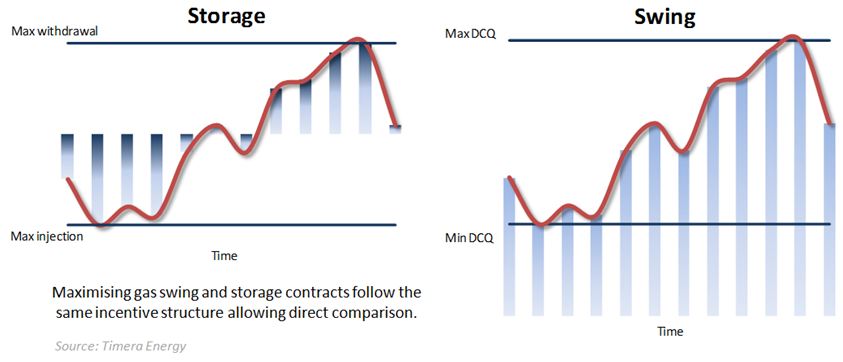
Note, that swing contracts often have complicating features requiring extensions to the general case described above. These features can range from the very simple (such as the inclusion of a baseload volume tranche) to the very complex (such as carry forward and make-up provisions or indexed contract prices).

Three broad categories of valuation methodologies

There are three broad categories of methodology commonly used to quantify the flexibility (or extrinsic) value of gas storage and swing.

Rolling intrinsic

This is the most transparent and intuitive methodology and as a result it often favoured by asset managers and traders. Flexibility value is managed by locking in observable forward curve spreads and then making (risk free) adjustments to hedge positions as prices move, in order to monetise market volatility. Planned injection and withdrawal decisions are adjusted to add additional margin.

A simulation based methodology can be implemented based on the following logic for each simulation:

t = 0

Optimise the storage facility against the currently observed forward curve and execute hedges to lock in intrinsic value.

t = 1 to T

Simulate the movement in the forward curve and re-optimise storage contract.

Calculate the value of unwinding existing hedges and placing on new hedges against re-optimised profile and execute profitable hedge adjustments.

The key points here are that at any point in time the hedge position matches the planned injection and withdrawal profile and the outturn margin will always be higher than the initial intrinsic hedge as adjustments are only made if it is profitable to do so.

Constrained basket of spreads

This methodology considers a storage contract as a series of time spread options to swap gas from one period (injection) to another in the future (withdrawal). The volume of available spread options is constrained by the physical characteristics (injection, withdrawal and space) of the contract or facility. The structure of the methodology is quite straightforward involving two steps:

Calculate a matrix of the spread option values of the different time periods (e.g. month). There are a range of spread option pricing models that can be used (e.g. Kirk or Margrabe) but all are likely to require volatility for each bucket and the corresponding cross maturity correlation.
Select the value maximising volume (“basket”) of spreads that is consistent with the injection, withdrawal and space constraints. This is typically based in a simple linear or mixed integer linear program.

The simple structure can be integrated into a simulation to capture how the structure of the spread options cascade in line with tradable products and how the facility is optimised in the prompt. Note, that in some cases more value can be created by allowing the model to trade linear products as well by effectively increasing the feasible volume of the spreads (e.g. for a given period a will allow the withdrawal legs of spreads can be offset against fixed injections increasing the overall available volume).

Optimal

There are several techniques in this category that are typically grouped together due to the similarity in their structure and underlying algorithms:

Trinomial Trees
Stochastic Dynamic Programming (SDP)
Least Squares Monte Carlo (LSMC)

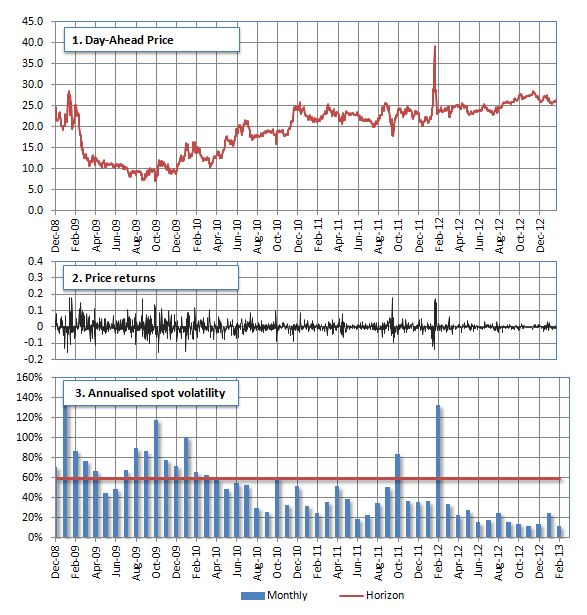
The common theme across the methodologies is that the optimisation decisions are in the spot (and as such, only require spot price models). In simple terms they are considered optimal as the decisions are aligned to the actual decision faced by the asset operator. That is, how much to inject and withdraw on a daily basis given imperfect foresight of future market prices but knowledge of spot price behaviour. For example: prices are volatile, if the spot price is high today it is also likely to be high tomorrow, prices are likely to drift back to an equilibrium level.

All three methodologies define a state space based on the time and inventory level. Then starting at ‘end of period’, use backwards recursion to determine the value maximising action (inject, withdraw and do nothing) for each state given consideration of spot price uncertainty. The methodologies differ in their treatment of spot price uncertainty and how it is incorporated into the calculation of the state transition value.

A comparison of the methodologies

The key advantages of the different methodologies are presented in the table below:

	Advantages	Disadvantages
Rolling intrinsic	Simple and transparent which promotes trust in results Consistent with the way many companies hedge and optimise flexibility (particularly seasonal) Can support a range of price processes Can be used to back test against historic prices (“what margin would I have made…”) Relatively easy to include market dynamics (e.g. product granularity and b/o spreads) add additional complexity (e.g. integration into portfolio valuation framework)	Not well suited to valuation & optimisation of fast cycle storage given limited spread liquidity & granularity in the prompt period Assumes “sub optimal” strategy of being fully hedged against expected profile (although this is a risk/reward trade-off) Relies heavily on the integrity of the simulation price process with care needed when choosing methodology (trade-offs involving complexity, calibration etc) Analytically complex and intensive Can be difficult to calculate meaningful Greeks
Constrained basket of spreads	Accessible (can be implemented easily in Excel), transparent and explainable Clear link between the methodology and hedging strategy and underlying instruments Simple parameter estimation (can directly use implied volatilities but generally need to calculate cross maturity correlations using historic prices) Easy to calculate Greeks	Doesn’t capture the true nature of the flexibility as the spread volumes are based on a deterministic optimisation of the inter-temporal optionality Undervalues within-month optionality as available spreads are generally constructed from tradable forward products (can significantly underestimate the value of fast cycle products).
Optimal	Captures the “true” nature the problem: Spot optimisation of the path dependency optionality Uncertain (stochastic) prices – assumes lack of perfect foresight of future market prices but knowledge of day on day price behaviour. Can be used as a decision support tool for complex hedging strategies (i.e. delta hedging) Can be used to value all types of storage/swing contracts (e.g. equally valid approach for seasonal and fast cycle storage).	Complex opaque methodology which can reduce transparency and faith placed in results Difficult to add extra dimensions (e.g. indexed contract prices or dual hub delivery optionality) Limitations of price models available for some methodologies (trinomial trees) but others support different methodologies through simulation (LSMC, SDP) Analytically intensive (especially for Greeks) Price model parameters generally not directly observable in the market.

Choosing a methodology

In our view, no single methodology is best. All approaches have strengths and pitfalls and an understanding of these is key to choosing the right tool for the job. There are however several key considerations to bear in mind:

Hedging and optimisation strategy: It is important that ensuring that actual (rather than theoretical) hedging and optimisation strategies are reflected in the methodology, i.e.:
- Alignment of the methodology to the actual strategy to be employed in value monetisation – it is no use an Origination team pricing off an optimal approach if the Trading desk will implement a rolling intrinsic strategy.
- Ability of the model to support the strategy (e.g. it will be critical that realistic deltas can be produced if a delta hedging strategy is to be employed).
Parameter estimation: Effectiveness and transparency of the methodology used are directly tied to the ease of input parameter estimation. The easier it is to observe or benchmark parameters against the market the better.
Diversification: Two or three views on value are better than one. The use of several methodologies alongside each other is likely to build a depth of understanding as the value & optimisation of flexibility.

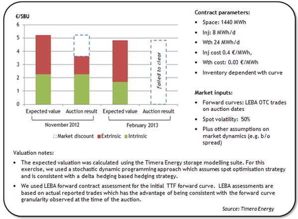
Finally it is important to recognise that the market will not pay for the expected value of an asset. A discount will be applied to reflect the costs and risks of monetising asset flexibility. Fortunately, the evolution of the market for gas flexibility products means that there are increasingly useful benchmarks (e.g. storage auctions, exchange traded options) to provide guidance on the market value of flexibility.

CCS – Will it take off anytime soon?

Posted on January 14, 2013January 16, 2020 by David Duncan

This week’s article is the next in a series of Guest Posts written by Howard Rogers, the Director of Natural Gas Research at the Oxford Institute for Energy Studies.

I published a paper in 2012 on the subject of CCS entitled (appropriately I thought) ‘Gas with CCS in the UK, Waiting for Godot?’. This line of research was prompted by a desire to get to the bottom of why such a potentially significant weapon in the quest for CO2 abatement, despite gaining the approval of all key climate change policy bodies, has to date not one commercial scale power sector application in operation globally.

Commercial vs technological challenges

The most common explanation is that of ‘technology challenges’. This is factually incorrect. Not only have the individual building blocks of the CCS chain been successfully employed in the upstream, petrochemical and refining sectors for decades, but commercial scale CCS chains have been deployed in the fields of natural gas processing and fertiliser manufacturing.

Whilst technological progress would certainly improve efficiencies and lower costs – especially in the CO2 separation stage – there are no barriers to making the process work, at scale, with coal or gas – fired generation plant. This is true whether we are considering pre-combustion (where the coal or gas stream is reacted with steam to form a mixture of CO2 and Hydrogen) or post-combustion (where coal or natural gas is used in a conventional generation plant and the CO2 extracted from the flue gas before it is vented in a stack). Pre-combustion configurations tend to require more complex process plant and lack the operational flexibility of post-combustion alternatives. This is likely to be important in the future where coal or gas fired generation with CCS could be required to provide flexible buffering or back-up to intermittent wind and solar generation.

The question of cost

We therefore come to the question of generation cost. As the following figure shows, the ‘levelised cost’ of generation from gas with CCS is similar to that of nuclear and onshore wind. Even the more expensive coal with CCS is more economically attractive than offshore wind. So if gas with CCS is similar in terms of generation cost with ‘mainstream’ low carbon generation technologies, why has it not been adopted at a commercial scale to date ?

Here I believe the issue is one of the commercial complexity of establishing a power generation with CCS ‘chain’. In order to successfully construct a commercial scale power sector CCS scheme it is necessary to ensure that the commercial arrangements for the power generation and CO2 separation, CO2 transportation and CO2 storage stages are covered by a ‘web’ of commercial agreements which appropriately apportion risks and rewards along all stages of the CCS chain. As current wholesale power market prices are set by unabated fossil fuel generation with currently only weak CO2 cost signals, it would be necessary that governments provide a level of assurance, not just on future power generation revenue, but more specifically on the difference between generation revenue and fuel costs. This is a level of complexity which has never yet been attempted in power markets which until recently have been run under an orthodox market framework.

Chart 1: UK Levelised Cost of Power Generation (Current Day Costs)

Source: Author’s calculations based on cost and operational estimates by Mott MacDonald. Assumptions: Gas price $10/mmbtu, coal price $90/tonne, CO2 price $64/tonne, 10% discount factor. Coal and Gas assumed 90% load factors.

The attraction of CCS

The enduring dilemma is that however difficult it may be to construct a workable commercial and subsidy framework for CCS – it represents a potentially very significant source of low carbon generation. Although the commercial arrangements for building offshore wind are more straightforward, ultimately gas with CCS may offer a more cost effective alternative to consumers. Another factor in favour of CCS is the challenge of ensuring system stability as installed capacities of wind generation become significant. Until a viable or affordable means of power storage is developed, wind power must be backed up by a controllable, flexible alternative means of generation. This could be hydro, coal or gas fired generation, but if it is the latter two, this may make it difficult to meet longer term carbon targets. Gas or coal with CCS could be an alternative to excessive levels of wind generation and a flexible complementary back up to wind if used in a post-combustion CCS configuration.

In conclusion, CCS is a technology which offers significant potential in helping society achieve decarbonisation of power generation. While technological progress can reduce the cost and improve the efficiency of CCS, it does not represent a barrier to successful implementation. The complexity of the commercial agreements and subsidy mechanisms require to support CSS investment in the context of a market-orientated power sector is the key challenge. However, absent breakthroughs in affordable power storage technology or other large scale ‘controllable’ low carbon generation, gas and coal with CCS must at some point be embraced if carbon goals are to be achieved, due to the shortcomings of wind and solar.

Whether the UK government has the drive and commitment to ‘see it through’ this time around is debatable. However if society remains committed to decarbonisation goals and breakthroughs elsewhere are not forthcoming, CCS is likely to remain an area whose undoubted technical viability and scalability will challenge those tasked with designing a framework to facilitate the necessary investment for at least the next few policy iterations.

An integrated transatlantic seasonal gas storage market?

Posted on January 7, 2013January 16, 2020 by David Duncan

European seasonal gas price spreads have been crushed over the last 5 years, falling towards 1 €/MWh. New sources of flexible supply, subdued demand and ample portfolio flexibility have driven the summer/winter price spread well below the level required to support construction of new seasonal storage capacity (7+ €/MWh).

But owners of seasonal flexibility (e.g. storage/swing) who are looking for a recovery in spreads will not take any comfort from the spread environment in the US. Indeed as the decade progresses, the US may start to export its underutilised seasonal flexibility, placing further pressure on summer/winter spreads in Europe.

Seasonal spreads … looking on enviously from across the Atlantic

These are difficult times for European storage capacity owners, but life is even tougher in the US. The glut of gas that has flooded onto the US market since the evolution of unconventional gas production has driven virtually all shape out of the US forward price curve. A forward curve comparison of NBP vs Henry Hub price shapes is show in Chart 1.

Chart 1: Current US and UK gas forward curves

Source: ICE (NBP) and CME (Henry Hub).

The value of seasonal storage capacity has fallen dramatically as a result. Indeed it has fallen to the point that storage capacity is being used to ‘warehouse’ gas (as an alternative to traditional seasonal cycling) as a bet on future price rises. Rising US natural gas prices are to an extent priced in, as can be seen by the relatively steep contango of the at Henry Hub gas curve in Chart 1. This is supported by an increasing production cost base for unconventional gas and the prospects of significant volumes of US LNG exports from the middle of the decade. Chart 2 illustrates the increasing trend in warehoused US gas volume.

Chart 2: North American Aggregated Gas Storage inventory

Source: The Impact of a Globalising Market on Future European Gas Supply and Pricing. Howard Rogers (OIES).

European spreads are close to historical lows, but US storage capacity owners would no doubt be looking at current NBP and TTF spread levels with envy.

Exporting seasonal flex from North America to Europe?

The transatlantic seasonal spread differential creates the interesting prospect of US storage capacity being used to provide seasonal flexibility to Europe via LNG exports. The seasonal profiling of US LNG exports to Europe is no forgone conclusion and a couple of key conditions would need to be satisfied for US exports to have a significant impact on seasonal spreads in Europe:

Firstly, enough US liquefaction capacity would need to be approved and built to allow a significant seasonal export flow of gas out of the US in response to transatlantic price differentials
Secondly, for gas to flow on a seasonal basis, the transatlantic price differential would need to converge towards the variable processing and transport costs to export gas to Europe (under the current NBP vs Henry Hub price spread, gas would flow baseload out of the US)

In other words US LNG export capacity would need to be unconstrained for it to be utilised for seasonal profiling of gas into Europe.

If the conditions are in place for transatlantic seasonal arbitrage, this will be driven by the within year price differentials between Europe and the US which may lead to changes in the utilisation of North American storage capacity. But the US gas market structure should ensure that any arbitrage value will be monetised given a liquid market providing sharp and responsive market signals and non discriminatory access to storage capacity at market prices.

Impact on the European market

It is important to note that transatlantic spread arbitrage would not have a meaningful impact until later in the decade, given the volume of new liquefaction capacity required to support profiled export flows. It is also likely that logistical complexities and shipping times will limit the role of US export profiling to the provision of seasonal flexibility. But if the right conditions fall in to place, the pent up flexibility in the US gas market could provide another blow to the value of existing seasonal flexibility in Europe as seasonal price differentials are further arbitraged away.