A framework for understanding European gas hub pricing

Posted on November 4, 2013January 16, 2020 by David Duncan

What drives the pricing of gas at European hubs? Oil indexation, long term contracts, LNG flows, Russian supply, interconnection, swing, storage… or all of the above and more. This is a problem that asset owners, investors, traders and risk managers grapple with on a daily basis given its importance as a driver of asset and portfolio value. But understanding European hub pricing dynamics does not require terabytes of data and a super computer. At a basic level it is a problem that can be tackled in your head.

There are two important considerations that can greatly simplify hub price dynamics:

Grouping sources of supply with similar pricing and flow dynamics
Focusing on the flexible volumes of gas that drive hub pricing at the margin

The first of these tasks is helped by the fact that most sources of European supply are under long term contracts that use a similar structure. The second task is assisted by the fact that only a relatively small volume of total European supply actually has the flexibility to respond to changes in market price.

The traditional approach to analysing gas market pricing is to build a ‘bottom up’ view encompassing a detailed representation of fields, pipelines and contracts. In this article we challenge that approach. The growing complexity of interconnected gas markets is eroding its validity.

Instead we present an alternative framework for understand hub pricing. At its simplest level this can be used as a qualitative frame of reference – i.e. tackled in your head. Or it can be extended to numerical analysis with varying levels of complexity. But importantly there is no substantial time or cost hurdle in starting to apply the framework logic.

Where the traditional approach breaks down

The traditional view has been that complex modelling is required to do justice to an understanding of European gas pricing dynamics. A detailed view is required of the characteristics and costs of fields, contracts, import infrastructure, transmission, storage etc. This means lots of data and a large and complex model.

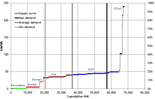
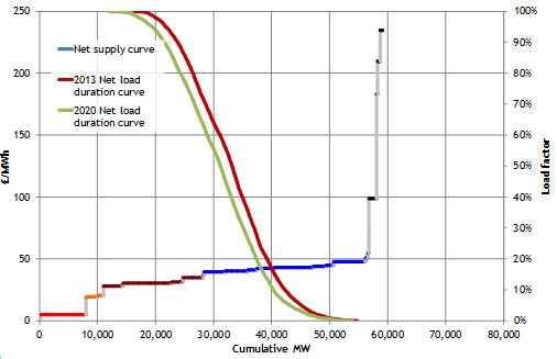
This bottom up supply and demand modelling approach works relatively well in power markets where price dynamics are primarily influenced by production costs. Transparent installed plant capacity and efficiency data combined with observable fuel costs mean developing a view of the power supply curve is relatively straightforward.

But the important difference with the European gas market is that most gas comes into Europe under long term contracts. So contractual pricing and flexibility are key drivers of physical flows and hub pricing dynamics. By contrast, contractual positions can largely be ignored in power market analysis where pricing dynamics are focused on variable production cost.

The traditional bottom up supply and demand analysis approach may have had its place when gas markets were relatively isolated (e.g. tackling the UK market on a standalone basis). But the European gas market is now a highly interconnected set of hubs across a complex range of physical infrastructure. Hubs are also increasingly influenced by global pricing dynamics. Trying to represent this complexity in a detailed bottom up model has two key flaws. The detail erodes transparency as to the real drivers of gas flows and pricing. And genuine insight is lost in the noise created by trying to capture the complexity of detail.

Grouping sources of European gas supply

To understand hub pricing dynamics it helps to start by drawing a ring around the European countries that have direct access to hub liquidity. The boundaries of this ring are somewhat arbitrary depending on focus, but broadly include North West, Central and Southern Europe. Within this boundary, European gas supply can be grouped into several key sources by geography as illustrated in Diagram 1. The diagram illustrates volumes by supply source based on 2012 gas flows.

Diagram 1: Sources of European gas imports

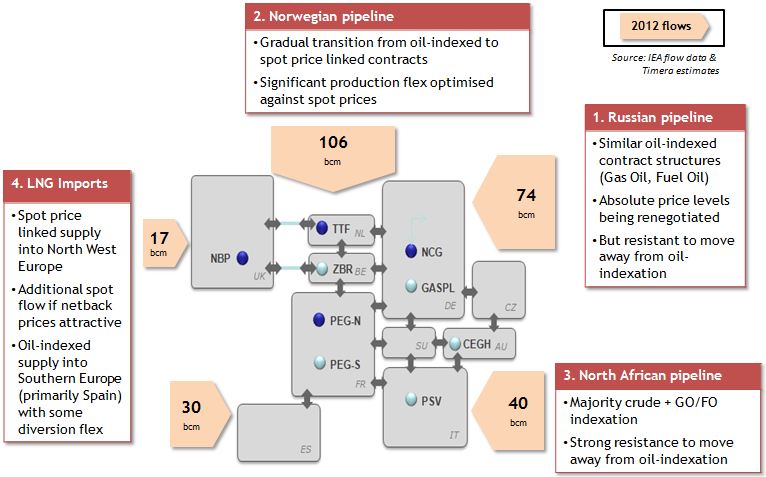
Note: Diagram and gas flows based on a European hub zone boundary that covers UK, BE, NL, FR, DE, CZ, AU, CH, IT & ES.

The following is a brief summary of each source of supply:

Russian supply – imported under long term supply contracts of a relatively consistent structure, incorporating (i) indexation to oil products (ii) with some volume flexibility but (iii) a take or pay constraint.
Norwegian supply – which can be split into two components:
- Long term oil-indexed supply contracts (on a similar basis to Russian supply).
- Supply that flows based on spot price signals, incorporating (i) hub indexed supply contracts and (ii) uncontracted Norwegian production.
North African supply – primarily import contracts into Italy and Spain on a similar pricing and flexibility basis to Russian gas (although with a greater influence of crude indexation and generally higher contract prices).
LNG supply – which can be split into two components:
- Long term oil-indexed supply contracts (primarily into Southern Europe).
- Supply that flows based on spot price signals, incorporating (i) hub indexed supply contracts into North West Europe and (ii) global LNG spot market supply (i.e. cargoes that flow into Europe based on spot price signals).
Domestic production – dominated by declining field production in the UK and Netherlands.

The other key supply dynamic that is not captured in these five categories is gas storage capacity. This is not to say storage should be ignored – it can in fact be a very important driver of hub pricing dynamics. But it makes more sense to think of storage capacity as enabling the movement of gas between time periods, rather than as an outright source of supply. Seasonal storage acts to move gas from lower priced summer periods to higher priced winter periods. Fast cycle storage acts in a similar fashion but over a short time horizon.

The geographical groupings of supply sources set out above are defined primarily on contractual rather than physical characteristics (although uncontracted sources are also captured). This enables a focus on the commercial decisions that drive the pricing and flow of gas, rather than trying to capture the detailed complexity of physical assets and infrastructure. The logic of these groupings will become clearer as we explore how flexibility drives pricing.

Types of supply: flexible vs inflexible

Gas supply volumes are either flexible or inflexible. Flexible supply can respond to changes in hub pricing, with flows based on the relationship between hub prices and contract prices (or an opportunity cost alternative in the case of storage). But the majority of European gas supply is inflexible, i.e. supply volumes are insensitive to changes in hub prices. This characteristic is key because it greatly simplifies the task of understanding hub price drivers.

Inflexible supply falls broadly into three categories that make up around 75% of European supply:

Pipeline contract take or pay volumes – Virtually all long term pipeline supply contracts into Europe contain provisions where buyers must pay for gas volumes (typically 80 – 90% of annual contract quantity) regardless of whether gas is taken.
Destination inflexible LNG contracts – Supply contracts into Southern Europe have traditionally had fixed destination clauses that prohibit the diversion of gas (although a number are being renegotiated).
Domestic production – With the exception of a small number of fields, production within Europe is largely insensitive to price.

It is important to account for these inflexible volumes in developing an overall view of the supply & demand balance across Europe. These volumes will essentially flow regardless of the absolute hub price level (although several tranches are profiled within year and have an influence on seasonal price spreads). But in terms of understanding the drivers of hub pricing dynamics, inflexible volumes sit a long way down the list of priorities.

Much more important are the volumes of flexible supply that are responsive to price. These are summarised in the following table:

Flexible tranche	Impact on hub pricing
Pipeline contract swing volumes	Contract owners optimise swing volume flexibility in pipeline contacts as a function of contract prices and hub prices. Broadly, contract lift is minimised to take or pay levels if contract owners can source their incremental gas requirements for less at the hub (contract price > hub price) and contract lift is maximised if it is cheaper to do so (contract price < hub price).
Uncontracted pipeline import flexibility	Focused on Russian and Norwegian production given North African supply constraints: Norway typically flows gas to spot price signals within a target production range. Russia is likely to require hub prices at or above existing oil indexed contract levels before flowing additional uncontracted gas.
Spot and divertible LNG supply	Divertible LNG supply contracts typically flow based on the opportunity cost of LNG in the global spot market (i.e. hub prices need to be above global spot prices adjusted for shipping, risk premiums and transaction costs), although portfolio dynamics may also influence diversion economics. Spot LNG cargoes flow into Europe if hub prices are greater than prevailing netback global LNG spot prices (as was the case in 2009-10). One notable exception is Qatar which currently manages a ‘strategic’ flow of spot LNG cargoes into North West Europe, in order to avoid putting excessive downward pressure on the Asian spot price (a threat to its long term contracting goals).
Gas storage	Storage capacity provides the flexibility to move gas between different time periods (e.g. summer to winter). The exercise of this flexibility is driven by the opportunity cost of flowing gas in different periods, which is in turn a function of the other flexible supply sources set out in this table. So storage acts to smooth seasonal shape and volatility in hub prices, but it is not a primary driver of hub price level.

Hub prices move based on the changing intersection between demand and supply. Given demand is relatively insensitive to price, it is supply flexibility that plays the central role in determining how prices evolve at the margin. So a solid grasp of hub price dynamics can be built around an understanding how the different sources of flexible supply interact to drive marginal pricing.

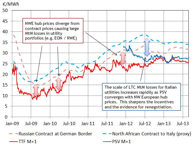
In order to do this a view of the pricing of each flexible supply source is required. Although there are many individual supply contracts that determine this, the fact that each flexible supply source uses a similar pricing structure makes life easier. Price proxies can be developed relatively easily, for example for Russian, Norwegian and North African oil-indexed supply (see here for an explanation of how). Alternatively if you prefer to steer clear of spreadsheets, you can gain a reasonable understanding from forward market prices and published contract benchmarks, for example for the German border price of oil-indexed contract imports.

Pulling everything together

So far we have talked about (i) geographical groupings of supply and (ii) different types of flexible supply. The picture comes into focus when we combine these two views to define the main individual tranches of flexible gas supply. It is the commercial dynamics of these tranches that are the primary driver of hub pricing dynamics.

Of the flexible sources of supply, pipeline contract swing is of principle importance. Russian and Norwegian oil-indexed contracts are particularly important as a provider of swing flex into Germany. Utilisation of this swing flexibility tends to anchor European hub prices within a band around oil-indexed contract price levels.

This price band is somewhat flexible, but it is also resistant. It can be stretched by prevailing supply and demand dynamics, but the further prices deviate from oil-indexed benchmarks (e.g. the German border price), the stronger is the force acting to pull prices back. As hub prices fall below oil-indexed contract prices, contract owners utilise swing to pull back on contract volumes which supports hub prices. As hub prices rise above oil-indexed levels, swing gas flows increase acting as price resistance.

Norwegian uncontracted production flexibility also plays an important role. Norwegian flows are a key source of seasonal flexibility as well as an equalising force across hubs (given multiple delivery points across North West Europe). Norway also holds an important strategic card in being able to pull back on production to support hub prices in periods of oversupply.

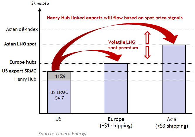
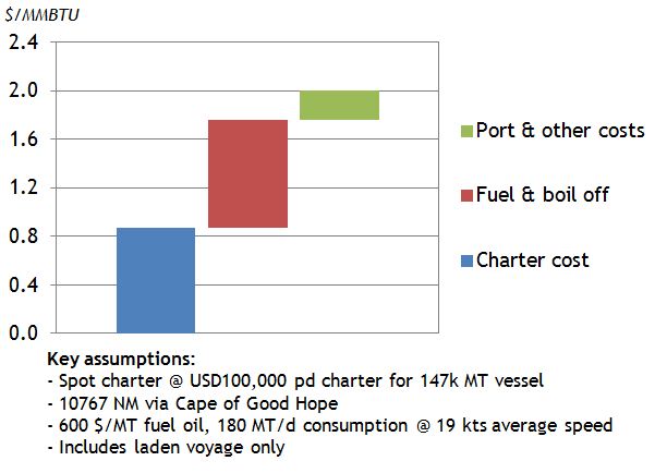
Flexible and spot LNG supply is currently of less importance to European hub pricing. The prevailing structural Asian spot price premium means diversion flexibility is being fully utilised to send cargoes east. But with volatile spot prices, this situation can change at short notice e.g. the temporary LNG flows back into Europe in summer 2012.

Next week we apply the framework

The logic set out above describes the basic elements of a framework to understand European hub pricing. This is built around the interaction between the flexible tranches of supply that drive marginal pricing. At a summary level these are factors that you can grapple with in your head. If you want to dig deeper, a more dynamic representation of the framework can be developed in a spreadsheet relatively easily. We have taken it a step further again and developed a more detailed framework model, but this is no prerequisite.

Next week we focus on the more practical application of this framework, using examples to illustrate how tranches of flexible supply move hub prices. Importantly we also look at the strategic considerations of the key players with significant market power, the Russians, Norwegians and Qataris. To do this we develop a simple ‘supply stack’ view of European flexibility. We then use the framework and supply stack view to illustrate the commercial dynamics driving hub price evolution.

Strategic negotiation with portfolio assets in play

Posted on October 28, 2013January 16, 2020 by David Duncan

This is the third and final in a series of articles on commercial negotiation of long term energy contracts, written by Nick Perry.

In the first two parts of this series we looked at how out-of-the-money long term energy contracts (LTCs) give rise to commercial tensions. We considered how these can either degenerate into wasteful commercial conflict or, more constructively, act as a catalyst for win-win renegotiations. We also considered the scope for creativity in recasting the contract across several of its many dimensions, allowing the distressed party to trade for some relief against its main source of financial pain, and enabling both sides to avoid the uncertain outcome of arbitration or the courts.

In this final article of the series, we extend this lateral thinking even more widely, to look at opportunities for commercial tradeoffs at a portfolio level.

Broadening the scope

We have already observed that by their very nature, LTCs are complex and multi-dimensional. This provides fertile ground for creative commercial thinking and, in particular, for win-win opportunities to be found. These often arise as a result of asymmetries in the positions of the two parties: their respective costs of capital; their assessments of extrinsic value; their tax positions; their varying abilities to manage risks; their trading capabilities etc.

In the same vein, it is usually the case that the parties to large energy LTCs are companies with extensive portfolios. These often range widely across regional energy sectors (utilities with generating fleets, gas assets and infrastructure investments) or international markets (oil and gas players with widespread interests), or indeed both.

Leveraging the portfolio

Large companies rarely see themselves as static: they generally have strategic goals that include transition over time away from, say, one traditional class of assets or geographical location towards another. Their counterparty in an LTC may very probably have assets that could be of interest to them in their longer-term objectives: and in the 21^st century most assets ‘have their price’.

Open-minded consideration of the two portfolios across the negotiating table may reveal useful differences in valuation – be that cash or strategic value – that can be traded on, in exactly the same way as terms within the LTC but on an even larger and more fruitful scale as illustrated in Diagram 1.

Diagram 1: Creating value by expanding negotiation creativity and scope

The key requirements to turn this from a theoretical prescription into a practical source of significant value are several:

Creative and experienced negotiators, deal structurers and advisers
A comprehensive and flexible analytical capability to identify and value opportunities
Open-minded corporate management, willing to consider creative solutions

Companies should resource negotiations appropriately to the amount of value at stake. These can be among the largest sums that will ever be contested across their negotiating tables.

Companies that know the score

The energy companies that are probably most familiar with this approach are E&P players in the oil and gas sector. They often have very different legacy portfolios specialities. For example, one may have an exploration bias, a US market orientation, and strongly prefer gas assets over oil; another may have offshore specialities, its own refineries, and favour already-producing oil plays in developing markets.

Their risk management precepts also place value on portfolio diversification; and they are well-versed in joint ventures, ‘farming-in’ and ‘farming out’ assets. Asset swaps are a familiar feature of their commercial repertoire. For such companies, their non-core assets are always potentially ‘in play’, and can serve to add a depth of possibilities to a commercial forum that was initiated by the need to renegotiate an LTC.

Examples of the portfolio approach

Companies from other traditions do well to emulate this open-minded commercial approach, and some have done this successfully. Good examples include:

E.ON, which has exchanged European downstream positions and midstream assets with Gazprom in exchange for upstream assets in Russia
BASF, which has packaged gas LTCs with assets and marketing ventures in deals also with Gazprom

Perhaps the most comprehensive example of a successful portfolio approach to solving distressed LTCs is that of the former British Gas Corporation (BGC), and its offshoot Centrica in its first years of existence after de-merger from BGC in the mid 1990s. At that time BGC was in a classic LTC squeeze, having over-bought gas in a series of GSAs at prices that were many billions of pounds out-of-the-money after the UK gas price collapse of 1994-5.

In order to give its corporate restructuring the best chance of success, BGC and later Centrica entered a series of difficult renegotiations with the key gas producing companies that were the counterparties to their GSAs. They were prepared to consider any contractual structure, and indeed settled on a wide range of different solutions. Some deals were bought out for cash; some with changes to the detailed terms of the GSAs; and others involved assets from BGCs own portfolio of UKCS assets.

In less than 2 years they negotiated out the most economically damaging prices in their portfolio under more than a dozen LTCs – a very commendable timetable, given how long some LTC counterparties take to renegotiate a single GSA. (For completeness it should be noted that the UK government made clear to all the parties concerned that they were expected to make constructive progress in these sessions, and itself contributed expeditious treatment of the several complex tax issues involved.)

Negotiating with perspective

Out-of-the-money LTCs can be a source of substantial damage to energy companies, with severely out of the money contracts sometimes proving fatal. Attempts to re-negotiate contracts can be extremely fraught. Too often a one-dimensional, zero-sum, win-lose approach is taken to contract negotiation. But a creative commercial approach that is allowed to range over as wide an area as possible – within the LTC itself and sometimes even more widely across the portfolio – can identify win-win opportunities that facilitate better outcomes for both parties.

Gas plant & renewable penetration: a UK case study

Posted on October 21, 2013January 16, 2020 by David Duncan

The increase in renewable capacity is eroding gas plant generation margins across Europe. At the same time there is an increasing system requirement for gas plant flexibility to support renewable intermittency. This paradox is challenging the orderly operation of wholesale power markets in Europe. But it remains unclear how intermittent renewable and gas-fired plant will happily coexist.

In this article we focus on the interaction between renewable and gas capacity by exploring their impact on supply curve dynamics. The issues are similar across most European power markets, but we have chosen the UK as a case study given its tight capacity margin and security of supply issues. The UK response to gas plant remuneration may well form the blueprint for other European markets to follow.

Supply curve transformation

Commodity prices and government policy are conspiring against gas plant across Europe. The precipitous fall in coal prices over the last two years has resulted in coal plant sitting clearly ahead of gas plant in the generation merit order. At the same time, government support for low variable cost renewable capacity is eroding gas plant generation margins. These factors are best understood by considering their impact on the generation supply curve. While the effects are similar across most of Europe, we focus on the UK market as an illustration.

Chart 1 shows the UK generation supply curve. UK plant are ranked by short run marginal cost based on forward fuel and carbon prices for the 2013-14 gas year (Oct 13 – Sep 14). The volume of intermittent renewable capacity is de-rated for average plant load factors (e.g. average wind conditions). So the chart shows a snapshot of supply given average conditions across the year.

Chart 1: UK supply stack (2013-14)

Source: Timera Energy. Note: Supply stack reflects average plant & interconnector availability. Actual plant & interconnector operation will differ at any specific point in time depending on availability, system requirements & market conditions.

Government support is expanding the low cost tranches of renewable capacity (wind, solar, biomass) at the left of the supply curve. This pushes the market price setting tranches of gas and coal capacity to the right, reducing thermal plant load factors. As a result, demand (illustrated via max, average and min annual levels) is met by cheaper plant, dragging down wholesale power prices. Lower load factors and lower power prices are eroding gas plant margins and value.

Looking at the problem through a different lens

It is difficult to get a clear picture of the impact of renewable intermittency by looking at the supply curve snapshot in Chart 1 which only shows annual average load factors. A different approach is required in order to appreciate the impact of swings in the output of intermittent capacity. It is more helpful creating a supply curve net of uncontrollable generation (e.g. wind, solar and interconnectors). Uncontrollable generation can then be netted of system demand to generate a net load-duration curve as illustrated in Chart 2.

The left hand vertical axis in Chart 2 again shows the marginal cost of plant as for Chart 1. But the load duration curve which is overlaid, is measured against the right hand axis and shows the range of system demand (net of uncontrollable generation) from the lowest hour in the year (top left = 100%, ~56GW), to the highest hour of the year (bottom right = 0%, ~17GW). The red net load duration gives an indication of current conditions based on actual 2012 demand, wind and interconnector flows.

Chart 2: UK supply stack net of uncontrollable generation (2013-14)

Source: Timera Energy. Note: 2012 relationship between demand, wind, hydro and interconnectors has been used to project net load duration curve. Load factors are indicative only.

The advantage of this adjusted view of the supply stack is that it gives a much clearer indication of how thermal plant are required to meet net system demand. An indication of annual load factors for different plant can be measured against the net load duration curve. For example it can be seen that:

Only the most efficient coal plant are required to operate baseload
Newer CCGT plant are currently only running mid-merit (~50% annual average load factor)
About a third of UK CCGT capacity is currently running at very low or zero load factor (i.e. only really operating for balancing and reserve purposes)

The impact of adding another 10 GW of intermittent renewable capacity to the UK stack this decade is illustrated with the green net load duration curve. Compared to the red curve, the green net load duration curve stretches to the left as average renewable output increases, but peak net system demand (bottom right = 0%) is largely unaffected.

Adding wind and solar capacity reduces average net system demand across the year. But there are still hours in the year when the wind doesn’t blow and the sun doesn’t shine. New renewable capacity has little impact on the volume of backup gas plant capacity required to maintain security of supply. It also increases transmissions stress and system balancing issues. So in order to maintain security of supply, gas plant needs to be adequately remunerated for providing flexibility support.

The gas plant owner’s dilemma

Saying that the market needs to remunerate gas plant may sound like cold comfort to asset owners currently being battered by depressed plant margins. After all there is a long history of markets making a fool of economic theory. But as renewable capacity continues to expand across Europe, there appear to be 3 potential outcomes for gas plant remuneration:

Market remuneration: Gas plant returns increase in the fewer hours of the year that plants operate i.e. there is an increase in market and balancing mechanism volatility and ‘super peak’ pricing. While the market may deliver this outcome if left alone, regulatory authorities may not tolerate the associated price volatility.
Capacity/reserve payments: Regulatory authorities step in to provide support for gas plant via new revenue streams outside the wholesale energy market e.g. via capacity market and/or supplementary reserve payments. This looks to be the route the UK will pursue.
Under remuneration: There is inadequate remuneration for flexible gas plant, causing plant closures and a tightening capacity margin. This describes the current conditions across much of North West Europe given surplus capacity, although as thermal capacity closes 1. or 2. will eventually need to happen if security of supply is to be maintained.

Support for renewable capacity is set to continue to erode gas plant load factors. But the key question for gas plant owners is how incremental flexible capacity will be remunerated going forward. Via wholesale market spreads and volatility, via a capacity market or via balancing and reserve payments. The UK, given its relatively tight capacity situation, is the ‘canary in the coal mine’ for European power markets. In an article to follow, we will consider how the uncertain evolution of plant remuneration impacts gas plant valuation.

US exports are a big deal for global gas pricing

Posted on October 14, 2013January 16, 2020 by David Duncan

US LNG exports are firmly on the gas industry radar. But the primary focus to date has been on whether US LNG is cheap vs alternative sources of supply such as Australia and East Africa. While this focus is understandable from a competitive perspective, US exports are more than just another source of global supply.

The structure of US supply contracts is fundamentally different to that of conventional LNG supply. Importantly, US LNG supply is hub indexed and inherently flexible. As a result, the ramping up of US exports mid-decade is set to significantly impact global LNG pricing dynamics.

US export contracts vs conventional LNG supply

US supply contracts are structured as a liquefaction capacity option rather than a firm commitment to take a volume of cargoes. This capacity option is exposed to the spread between Henry Hub prices and the shipping cost adjusted netback spot prices that can be achieved selling gas into the global market.

Fixed cost: The fixed fee (or option premium) component of cost is a capacity fee. This is designed to cover the costs of liquefaction terminal development. The 2.25 $/mmbtu fixed fee in the first export contract from Sabine Pass between BG and Cheniere, gives a reasonable indication of the cost of brownfield liquefaction development at an existing US regas terminal. Fixed fees in export contracts signed since this have been closer to 3 $/mmbtu, although it will be interesting to see if these levels can be maintained as export project competition hots up.

Variable cost: The fixed fee is important from a total supply cost perspective. But once an export contract is signed, this cost is sunk and therefore becomes largely irrelevant in influencing commercial decisions around the flow of gas. The variable cost of exports at Sabine Pass is structured as a percentage premium on top of the Henry Hub price. So the short run marginal cost (SRMC) of exported gas is 115% times the Henry Hub price (about half of this premium covers the actual cost of gas used in the liquefaction process).

Importantly there is an inherently high level of flexibility in export contracts. Flexibility to hedge price levels at Henry Hub. But also flexibility to deliver exported gas to whatever location offers the highest netback spot price. This is a very different structure to traditional fixed destination clause oil-indexed LNG supply contracts.

US export contract flow decisions

The flow decision for US export contracts will be driven primarily by two factors:

The variable cost (or SRMC) of US export contracts i.e. Henry Hub plus the costs to get LNG onto a vessel (primarily liquefaction).
The netback global spot price signals that represent the market value for exported gas, adjusted for appropriate shipping costs.

As long market conditions are such that 2. exceeds 1. then US gas will flow into the global market, constrained by the volume of US export capacity.

On a variable cost basis, US exports are relatively cheap. Based on current Henry Hub forward prices, US export SRMC will be around 5 $/mmbtu mid decade, rising to around 7 $/mmbtu by the end of the decade (given forward curve contango). Add $1.00-1.50 for shipping to Europe and $2.50-3.00 for shipping to Asia and these contracts are well in the money on an SRMC basis vs European (9-10 $/mmbtu) and Asian ($15/mmbtu) price benchmarks.

So barring the return of another major global gas glut (not out of the question, particularly later this decade), US export contracts should flow baseload. But given the inherent delivery flexibility in the export contracts, LNG will tend to flow to spot price signals, unlike most of the existing DES long term contracts into Asia.

That does not mean that flexible LNG contracts will always be physically diverted to the highest priced market. There are important liquidity, transactions cost and portfolio effects that will impact the actual flow of gas. But LNG spot price signals will represent an increasingly transparent opportunity cost for the contract owner, of the decision to flow gas to a particular destination. Whether that opportunity cost drives the actual diversion of gas, sale to a third party or internal portfolio re-optimisation will depend on the specific circumstances involved.

Watch out for the spot market impact

The volume of the first tier US export projects looks to be in the order of 45 to 60 mtpa (of a total ‘proposed’ volume in excess of 200mtpa). In a global market context (~240 mtpa) this is not an overwhelming volume when anticipated incremental demand growth is considered. However the volume of first tier US projects is large in the context of spot market pricing dynamics, given only around 20% of global LNG supply is currently flexible.

This significant increase in LNG volumes that flow to spot price signals is set to have two key impacts on global pricing as illustrated in Chart 1.

Chart 1: The impact of US exports on global spot price dynamics

US exports will act to:

Reduce global spot price differentials – given delivery flexibility, US LNG will tend to flow to the highest price market on a netback basis.
Reduce spot price volatility – US exports will increase the volume of flexible gas to respond to fluctuations in global spot prices, dampening volatility.

As long as US export capacity remains constrained, this will limit the extent to which Henry Hub becomes a key driver of long term contract pricing. However on a shorter term basis the influence of Henry Hub price signals on LNG spot pricing dynamics is likely to increase, even if US export capacity remains constrained.

Implications for LNG supply contracting

Commercial and investment decisions in the LNG market are currently being strongly influenced by prevailing market conditions. That is understandable in a post-Fukushima world of tight supply, large regional price differentials and constrained supply flexibility, factors likely to remain until at least the middle of this decade.

However many market players are looking to invest in or acquire LNG supply flexibility over a much longer time horizon. And given current market conditions, supply flexibility is expensive. In this context, understanding the impact of US exports on pricing dynamics and the value of flexibility is an important consideration. LNG exports are ultimately a factor working against the value of LNG supply flexibility.

Getting creative with long term contract renegotiation

Posted on October 7, 2013January 16, 2020 by David Duncan

This is the second in a series of articles on commercial negotiation of long term energy contracts, written by Nick Perry.

European gas contract re-opener negotiations are re-shaping the pricing and flexibility of gas flows into Europe. Re-opener discounted tranches of Russian gas are having a growing influence in setting marginal hub prices. Greater portfolio supply flexibility is being facilitated by the negotiation of spot indexation, take or pay volume reductions and LNG delivery flexibility. Most of these renegotiations are being triggered by concerns around contract price level. But as parties come to the negotiating table there is a lot more in play.

In the first article of this series we noted that long-term energy transactions, like other forward contracts, generally have a very small mark-to-market (MTM) value for both parties when the deal is first done. However, over time the contract can increase in MTM value very significantly for one side – and decline in value correspondingly for the other. We now consider how this potentially damaging commercial tension can be harnessed constructively to benefit both parties.

Getting to the re-negotiation table

Genuine commercially-motivated re-negotiations will typically occur when both the buyer and seller agree that ‘something has to change’. This may be even though the parties have very different views as to what this change should be before they get to the table. Clearly, for at least one party an extreme adverse MTM value-shift can be one such reason for seeking changes.

European energy contract re-negotiations are usually initiated via one of two routes, depending on the legal jurisdiction under which the contract was signed:

Contracts entered into under a Civil Code approach (found in most European, South American and non-English-speaking Asian countries), typically contain re-opener clauses that specify the conditions under which contract counterparties should come together to resolve a dispute.
Contracts entered into in a Common Law context (as found in most of the English-speaking world), typically do not have a formal contractual trigger for renegotiation, meaning that it is usually commercial incentives that bring parties to the table.

For those interested, a further analysis of Common Law and Civil Code context is provided in the breakout section below. Otherwise, we move straight on to the commercial considerations in contract negotiation.

Further analysis: A Layman’s Guide to Common Law vs Civil Code context

In a Civil Code context, conditions of extreme market movements or any other cause of material change in contract MTM value make it almost inevitable that re-negotiation will occur. By contrast, the Common Law legal tradition is for contracting parties to make changes to contracts only through bilateral (re-)negotiation, coming together for this purpose on a voluntary, ‘willing buyer, willing seller’ basis.

[Read more]

Under the Civil Code approach (found in most European, South American and non-English-speaking Asian countries) there can be circumstances in which a commercial court could intervene to impose a change in price and other contract terms: and one or other contract party could unilaterally approach the court for such a ruling – usually when they were in financial distress arising from the terms of the contract. In advance of such a situation (i.e. when the contract is first being negotiated) parties are naturally reluctant to leave their future commercial fate for a general commercial court to decide, and would prefer expert arbitration.

To avoid the courtroom, LTCs subject to Civil Code jurisdiction therefore generally contain ‘re-opener’ clauses which dictate conditions under which one or other party can demand that the contract be submitted for expert determination, which both parties agree in advance they will accept. These clauses will typically state a time-interval (e.g. 3 years) and a ‘threshold of pain’ (e.g. extent of change in market conditions) which must be met in order for one party to be able to call for arbitration unilaterally. It is usual for re-opener clauses also to require negotiations to be conducted in good faith prior to the suffering party invoking arbitration.

Common Law parties sometimes agree that foreseeable contractual disputes on minor matters are to be settled by arbitration; but it is very rare that they would allow arbitration to change something as fundamental as contract price, however extreme the market circumstances.

Likewise, under Common Law, the courts are generally unwilling to impose a change in contract price or other significant terms, even if the contract has become materially out-of-the-money for one party. So any re-negotiation will take place only because both parties feel they have something to gain.

Negotiation – Civil Code context: contract renegotiations follow a formal re-opener process. The potential paths through the re-negotiation of a long term gas supply contract are illustrated in Diagram 1.

Diagram 1: European long term gas contract re-negotiation map

In the diagram we take the extent to which the contract has become out-of-the-money (OTM), either ‘material’ or ‘immaterial’, as a proxy for the degree of pain being suffered by a contract party. Material represents MTM stress above the contractually defined ‘pain threshold’ to trigger a re-opener. If the buyer assesses the contract is OTM for itself we assume it will assess it as being correspondingly in-the-money (ITM) for the seller. It is worth noting however, that it will not always be that the buyer and seller agree in their assessments either of their own position or their counterparty’s.

There are broadly 3 potential situations that can arise:

1. No re-opener

If both the buyer and seller independently assess that the contract is (i) ITM for themselves, or (ii) OTM but only to an immaterial extent (i.e. below the ‘pain threshold’). Then they will not convene to re-negotiate (the grey area marked A in the diagram).

2. Negotiation

If the buyer and seller both agree that one of their positions is OTM to a material extent, then they will meet to renegotiate (areas B and C). This has been illustrated by the more proactive approach Statoil and Gas Terra have taken to renegotiating some of their ITM contracts with European suppliers (area C).

Interestingly, if both parties simultaneously consider the contract is OTM for themselves (and they might both be right!), they will also meet to renegotiate (area D) even though they may be seeing things differently. This can be the most fruitful circumstances for a win-win outcome!

An example of this is an oil-indexed European LNG supply contract with a fixed destination clause, which is OTM vs European hub prices for the buyer and OTM vs Asian LNG prices for the seller. Both parties win from cancelling the contract, or negotiating diversion rights such that upside is shared between the buyer and seller.

Of course, nothing guarantees that re-negotiations will succeed, and ultimately the case may go to arbitration (or the courts).

3. Arbitration

Arbitration tends to result when the buyer and seller disagree on the size/impact of the change in contract value. For example, if the seller is of the view that the contract is OTM for itself and the buyer rejects this assessment, the seller will invoke arbitration (area E): or vice versa for the buyer (area F). A prominent example of this is the recent arbitration cases between Gazprom and large European gas suppliers, where there has been a fundamental disagreement over the role European hub prices play in determining the long term value of gas.

Negotiation – Common Law context, there are typically no formal contractual drivers for the re-negotiation process, or recourse to arbitration or the commercial courts. What happens commercially will then be a function of the attitudes of the parties. If the ITM party is reluctant to engage, without a back-stop of arbitration sometimes the only ‘threat’ available is for the OTM party to hint at inability to perform the contract. In extreme circumstances some distressed parties have been known to default deliberately in order to trigger negotiations. There were several cases of this happening in the period 1995-98 in the UK, when the gas price collapsed and many contracts became significantly OTM. Needless to say, this often degenerates into litigation, and represents a failure of sound commercial practice.

It must always be a principle of good business that parties should at least meet to explore each others’ positions. Regrettably, in both Civil Code and Common Law contexts the ITM party often enters discussions with the time-worm attitude: what’s mine is mine, and what’s yours is open for discussion.

Identifying opportunities for win-win

When an OTM party comes to the table it will generally be self-evident as to what changes ideally they would like: at its most basic, a distressed seller will ask for a higher price and a buyer will want a lower. As we noted in Part 1, the counterparty must certainly have uppermost in mind a clear perception of what is at stake, not least when the LTC represents a hedge.

In consequence it can be all too easy to see the matter as a straight win-lose, zero-sum game: the buyer wants a lower price – how can that be other than at the direct expense of the seller? Unless there is a genuine prospect of the buyer’s bankruptcy (which would completely nullify the seller’s hedge), can the buyer’s appeal for a lower price be other than a charitable request (perhaps based on the business relationship)?

Nine times out of ten, for the seller to approach the situation from this limited perspective is culpably to ignore the scope for creative outcomes.

One of the most striking aspects of energy LTCs is how complex they are – inevitably so, as they must cover the wide range of contingencies which energy companies face. To contract administrators, complexity can be a nightmare! To the creative negotiator, however, complexity is a rich source of commercial possibilities.

At very least, LTCs will frequently contain terms such as price-indexation formulae and flexibility provisions (swing, take-or-pay, carry-forward etc). These represent multiple dimensions, all of which can be analysed for the value that lies in them. And whereas the buyer and seller will typically have the same view of the value of one unit of price, they may have quite different assessments of the value of, say, an incremental 10% of swing, or a switch from oil indexation to spot-gas indexation in the pricing formula. This has been illustrated in the recent renegotiated outcomes of many of Gazprom, Statoil and Gas Terra’s contracts with suppliers.

Thus, price may to some degree readily be traded for movement in one of the other basic dimensions of value, for example the price decrease may be bought with an increase in flexibility. Here it is very usual – and commercially helpful – for valuation of flexibility / optionality to vary widely between different players in the same market. This is often the source of great opportunity for a win-win negotiated outcome.

Getting creative

But this is only the start of the creative thought-process. At its most general we can assert that over time, even an LTC that seemed perfect to both counterparties when first negotiated will start to become less satisfactory in many details. Given the complexity and sheer length of tenor of energy LTCs, and the significant changes that take place in energy markets, this is inevitable. The buyer will have his list of various changes he would ideally like to make, ranging across the whole contract, and the seller will have his own – likely to be different in many respects, which is exactly what gives rise to potential for fruitful trade-offs.

Therefore, both parties, including the ITM party, should be approaching the table with a prioritised – and carefully evaluated – wish-list. The list of possibilities is endless, including entirely new contract terms, and the number of dimensions in play goes far beyond price and flexibility. Everything has a price, and constructive win-win trades should be possible between open-minded and commercially-creative counterparties. There should always be a commercial pretext for constructive re-negotiation.

Viewed in this way, when an LTC becomes materially OTM it is seen as a catalyst for all-round win-win contractual enhancement, in which the suffering counterparty can trade for some degree of relief against its main source of pain. This is the correct mind-set for companies approaching a re-negotiation.

But this is not the end of the story, and in the final article of this series we consider an even more wide-ranging perspective on energy contract re-negotiation.

Getting comfortable with CCGT extrinsic value

Posted on September 30, 2013May 12, 2020 by David Duncan

CCGT power plant valuation has traditionally focused on intrinsic value, the value of dispatching the plant against prices observed in the forward market. Any mention of the extrinsic (or flexibility) value of CCGT assets, resulted in nervous glances around the table. Extrinsic value was considered to be icing on the cake. Nice if you could get some, but unreliable and unbankable.

With the rapid decline in CCGT generation margins since 2010, Europe is now a different place. Support for intermittent renewable capacity has driven down power prices and cheap coal has displaced gas plant from the merit order. CCGT asset values have been written down as a result. But the value of CCGT assets has evolved not disappeared.

Intermittency is causing a structural increase in the requirement for system flexibility, in the form of responsive but lower load factor generation. CCGT assets are well placed to service this requirement. But the extrinsic value from plant flexibility now plays a central role in defining CCGT asset value. The owner of a newer CCGT may still have the ability to hedge some intrinsic value over peak periods, but an increasing portion of asset value is now extrinsic. For older CCGTs, 100% of value is extrinsic.

Deconstructing CCGT asset value

CCGT value is driven by the clean (or carbon adjusted) spark spread achieved by the plant. This spread is simply the difference between the market power price and the variable cost of operating the plant, calculated in any given period as:

clean spark spread = power price[€/MWh] – gas price[€/MWh] / plant efficiency[%] – carbon price[€/t] × plant carbon intensity[t/MWh]

Note: the formula above is for a European gas plant. Conversions (energy and currency) and the consideration of the Carbon Price Floor are required when calculating the clean spark spread for a gas plant in the UK.

A CCGT asset is essentially a strip of options on the spark spread. These options can be exercised on a very granular basis over a short time horizon ahead of plant dispatch, e.g. against hourly or half hourly price granularity in the spot market or even finer granularity in balancing markets. But monetising plant value based on short term optimisation alone, usually results in unpalatably high earnings volatility.

So where possible, asset owners will typically hedge plant exposures in the forward market. Exposures can be hedged on a forward basis by grouping the strips of plant options into a granularity that matches available forward contracts in the power, gas and carbon market. These forward hedge positions can then be adjusted in response to changes in market prices.

Extrinsic value of European power plant

The intrinsic value of a CCGT can be monetised with low risk, by hedging generation margin in the forward market and then dispatching the asset to fulfil the hedge. So hedging intrinsic value sets a floor for plant returns (ignoring plant outage risk for the moment). But the plant can also be ramped up to respond to periods where spark spreads move higher and ramped down during periods of zero or negative spreads. Extrinsic value is generated from the flexibility of the power plant to respond to changes in market prices.

European CCGTs currently have relatively little intrinsic value at current forward market prices. Sparkspreads range from slightly positive values in the UK, to pronounced negative values in markets like Germany and the Netherlands that are currently suffering from significant overcapacity. In other words the strip of CCGT plant spark spread options is only slightly ‘in the money’ in the UK and well ‘out of the money’ across much of Continental Europe as illustrated in Chart 1.

Chart 1: Intrinsic/extrinsic value split for European generation assets

Source: Timera Energy

Note: Chart 1 illustrates baseload ‘in the moneyness’ of different assets. Assets can also be hedged on a peakload basis, giving a slightly different picture, although the principles are the same.

A lignite plant which is deep ‘in the money’ at current market prices, has relatively low extrinsic value. Lignite plant flexibility is of little value, given healthy generation margins mean the plant is likely to be running anyway. But weak forward generation margins for CCGT assets mean that extrinsic value is very important.

Extrinsic value for a plant is highest when it is ‘at the money’ or when the plant spark spread is zero. At this point only small changes in spread are required for the asset to ramp up if the spread goes positive, or ramp down if the spread turns negative. Similarly, small movements in forward prices may open up a spread margin that can be hedged.

The key driver of extrinsic value is market volatility. The more volatile prices and spark spreads are, the higher the value of plant flexibility in being able to respond. It is this exposure to spark spread volatility rather than to the absolute level of spark spreads that has historically made CCGT investors nervous about extrinsic value.

Monetising extrinsic value

In order to appreciate how CCGT extrinsic value can be monetised, it is useful to build up a view of how asset returns can be monetised in the market. A more conservative CCGT monetisation strategy can be thought of in three tranches:

In periods when either baseload or peakload forward spark spreads are positive, intrinsic value can be hedged to protect the asset owner from downside risk.
As forward prices move, the owner can adjust and improve on existing forward hedge positions to increase asset returns. This can be achieved via a rolling intrinsic or delta hedging strategy that monetises forward market volatility.
In the prompt horizon approaching real time delivery, the owner can hedge price shape and capture additional value using the flexibility of the asset to respond to volatility in within-day and balancing markets.

The extrinsic value of a CCGT is not as easily observable on a forward basis as intrinsic value. There are also a number of practical challenges in monetising extrinsic value which need to be taken into account when quantifying plant value, e.g. market liquidity, risk capital and transactions costs. But monetising the flexibility value of a CCGT does not need to involve speculation or excessive risk taking.

What drives contract counterparties back to the negotiating table?

Posted on September 23, 2013January 16, 2020 by David Duncan

This is the first in a series of articles on commercial considerations in the negotiation of long term energy contracts, written by Nick Perry.

The European energy industry is navigating a period of intense re-negotiation of long term contracts. Rapidly changing market price dynamics have resulted in large swings in contract value and exposed unintended consequences of original terms and conditions.

The outcomes of gas supply contract negotiations with Russia and Norway are having a substantial bearing on the financial viability of a number of European energy companies. At the same time, LNG supply contracts are being redrawn to reflect the impact of changing price dynamics and the increased value of diversion flexibility in a post-Fukushima world. In the power market, long term tolling contracts have been transformed by a sharp fall in spark spreads, lower load factors and an increase in plant flexibility requirements.

Long term contracts (LTCs) of large volume, long duration and high nominal value are widespread in the energy business. But the greatest absolute (mark-to-market) value is usually to be found when, after several years, an LTC becomes significantly in-the-money for one party, and correspondingly out-of-the-money for the other. In such circumstances, commercial creativity allied to good analysis and negotiation skills become critical factors for turning destructive win-lose stasis into positive win-win dynamics.

In this first article of our series on long term contract negotiation, we consider how these dynamics can be identified and fruitfully exploited for significant added value.

Price risk is the primary driver of contract value shifts

When a forward contract is first transacted in a liquid market, its absolute mark-to-market (MTM) value is usually close to zero for each party. Liquidity and transparency combine to minimise the chances of there being any large sums lying around on the negotiating table. This is generally the case even when liquidity and transparency are only partial. For price-takers in a market, the initial MTM may even be (slightly) negative when the deal is struck.

Good negotiators can often find ‘win-win’ ways to create positive initial value for both sides; for example, when they are able to arbitrage different costs of capital or diverging assessments of extrinsic value. The more ‘plain vanilla’ a forward contract, the less likely there is for a genuine win-win to be available but conversely the more complex the deal, the more likely it is to be possible.

Even so, initial contract MTM values will be small, perhaps even very small, relative to the nominal sums involved. (Parties that claim to have created large positive initial value are generally marking the contract to their own portfolio or – worse still – to their forecasts of future spot prices.) This is not to find fault with the transaction, which may represent a very sound hedge, for example, or a satisfactory liquidation of a physical position; or even a speculative open position taken on with full understanding of the potential downside. For a market-maker or arbitrageur, a small positive value on an individual deal may represent exactly what they are in business to capture, transacting small positive gains continually, in high volume and at low risk.

However, the MTM of unhedged large deals can evolve significantly away from their initial small value – in either direction. This of course is Price Risk, the primary category of market risk, and is nowhere more acute than in energy, where volatility is high and long-term price shifts can be dramatic. In order to illustrate this point, it is useful to consider a simple case study looking at the impact of the rapid convergence of Italian PSV and North West European hub prices.

Case Study: PSV convergence and Italian supply contracts

Large European gas suppliers (e.g. E.ON, RWE) suffered sharp losses in 2009-10 as the financial crisis took hold. Gas hub prices plunged below long term oil-indexed contract prices and a rapid fall in gas demand left suppliers long gas against take or pay obligations.

Italian suppliers were somewhat insulated from the trouble in northern Europe as the illiquid PSV hub continued to move in line with oil-indexed contract prices. However market events suddenly turned against Italian suppliers in 2012. The release of capacity on the TAG pipeline allowed the flow of surplus gas from Baumgarten into the Italian market, resulting in the rapid convergence of PSV and NW European hub prices. The scale and pace of this convergence is illustrated in Chart 1.

Chart 1: Hub vs oil-indexed prices and 2012 PSV convergence

Source: LEBA, IMF and Timera Energy

The plunge in PSV hub prices has become a key factor impacting renegotiation of a number of Italian supply contracts. ENI has the largest exposure to long term oil-indexed supply contracts in Italy. Although ENI’s losses from PSV convergence have been painful, they have been the catalyst for some favourable contract renegotiation outcomes. ENI has not only gained significant contract price concessions from Gazprom since 2012, but has renegotiated supply contract take or pay levels and indexation to reduce portfolio risk. Edison, another big Italian gas buyer, has also used the PSV price move as leverage in successful contract price renegotiations with Rasgas (LNG supply into Rovigo) and Sonatrach.

As is often the case, contract price has been the primary driver behind renegotiation. However negotiations have focused on concessions around a much broader range of contract parameters, e.g. spot indexation levels and volume flexibility, as parties try to re-optimise contract terms for changing market and portfolio conditions.

Approaching the negotiation table

Rightly, the first considerations for a company identifying part of its portfolio as having high MTM will be:

how does this sit in terms of Price Risk, and in particular, does it represent a hedge for a correspondingly out-of-the-money portfolio component? If so, the value and commercial integrity of the in-the-money deal will need to be defended purposefully, leading to …
what is the credit position of the counterparty to the in-the-money deal ?, They are likely to be suffering financial pressures commensurate with the negative value the contract represents for them; but the original company cannot be indifferent to this counterparty’s ability to perform.

Assuming the credit situation is not (yet) at crisis-point, it would be wrong for the first party simply to be satisfied with the security of the position and do nothing. The potentially damaging, indeed possibly deteriorating, situation the counterparty faces is likely to generate commercial forces that will bring the parties eventually to the negotiating table. Wait too long, and a crisis may indeed develop. By contrast, a timely pro-active approach, firstly to analysis and then to creative commercial engagement, can pay very big dividends.

In the next article in this series we consider the nature of typical renegotiation dynamics and set out a framework for systematic development of the commercial potential.

Nick Perry is a Senior Associate of Timera Energy. He has worked on large structured energy transactions for over 30 years, both as a principal and a consultant.

Getting to grips with LNG shipping costs

Posted on September 16, 2013January 16, 2020 by David Duncan

The LNG shipping market is characterised by unusual terms such as ‘demurrage’, ‘ballast’ and ‘bunkering’. It features interesting conventions such as ‘canal transit costs’ and is impacted by the very real threat of modern day piracy.

While all of this is interesting trivia, these factors all play a role in determining the cost of moving gas between locations. The market for LNG vessels is a different animal to the more homogenous traded markets for delivered gas. The costs of shipping gas are determined by very physical considerations around logistics and constraints.

LNG shipping costs have an important influence on global gas flows and pricing dynamics. LNG shipping costs are a key driver of:

The value that can be generated from moving gas between different locations
The level of price spreads between regions across the global gas market

Shipping costs have played a particularly important role over the last two years in determining the cargo diversion decisions to higher priced markets, as global prices have diverged post Fukushima. They are also a key consideration in understanding to what extent global prices may converge in the future.

In this article we provide an overview of the build up of LNG shipping costs and their influence on gas flows and pricing. We will then follow up with an assessment of global LNG shipping supply and demand dynamics and the implications of these on shipping costs.

Shipping cost components

The key components that make up the cost of shipping LNG are as follows:

Chartering fee: This is the payment for securing access to shipping capacity by chartering a vessel. There are broadly three ways to secure access to shipping capacity: (1) own vessel capacity (2) time charter and (3) single voyage or spot charter. Spot charter rates are generally higher and certainly more volatile than longer term time charter rates. We will look in more detail at the drivers and evolution of charter rates in an article to follow.

Brokerage: Vessel charters are typically arranged through specialist brokers and attract a 1-2% fee.

Fuel consumption: The voyage fuel or ‘bunker’ consumption is directly proportional to the distance and speed of the vessel. This is typically the second largest cost component after the chartering cost. The added complication for LNG vessels is the different propulsion mechanisms and fuel burn options. Most LNG vessels can burn fuel oil, boil-off gas or a blend of both in their boilers. As a result the calculation of fuel cost is closely tied to that of boil-off gas. Natural boil-off occurs at a rate of approximately 0.15% of inventory per day and at times boil off is forced above this level to further reduce the fuel oil requirements. Some modern LNG vessels also have the ability to re-liquefy boil-off gas, keeping the cargo whole (and allowing the use of more efficient diesel engines). Calculation of the direct fuel consumption is fairly straightforward but the opportunity cost of LNG boil-off is also an important consideration.

Port costs: The components and level of the costs of loading and unloading at ports can vary widely depending on location. For example, ports in less stable regions can levy large security charges associated with ensuring the safety of the vessel.

Canal costs: Transit costs have to be paid for using the cross-continental Suez and Panama canals. Only a small fraction of the current LNG tanker fleet can squeeze through the Panama canal making the Suez is the most common canal transit. Suez canal transit costs are a complex function of vessel dimensions and cargo (laden voyages being more expensive) and LNG vessels are entitled to a 35% discount after which the costs are in the region of USD 300-500k per transit. The Panama canal widening project, due for completion in 2015, will allow up to 80% of LNG vessels to make the transit. This will reduce the distance from 16,000 to 9,000 miles from the US gulf coast to premium Asian markets. The impact on shipping costs to Asia is less clear as the tariffs have yet to be published. However, any reduction will increase the competitiveness and influence of Henry Hub priced US Exports on Asian pricing.

Insurance costs: Insurance is required for the vessel, cargo and to cover demurrage (liabilities for cargo loading and discharge overruns).

In order to get an understanding of how these components combine to determine the overall cost of an LNG voyage, it is helpful to consider an example. Chart 1 shows the shipping cost build up of a spot charter voyage from Nigeria to Japan.

Chart 1: Shipping cost from Bonny Island Nigeria to Sakai Japan

Shipping cost impact on diversion economics & regional price spreads

The calculation of an appropriate shipping cost between two locations depends on how the cost is going to be used. Calculating the shipping cost behind cargo diversion economics is easier than calculating the shipping costs that influence inter-regional price spreads.

Diversion economics

The diversion economics for a cargo owner are based on a set of known parameters. The diversion decision is focused on the cost difference between sending a cargo to Location A (e.g. Japan) as opposed to its original destination, Location B (e.g. the UK). The relevant shipping cost for the diversion decision is the true incremental cost of Location A over Location B.

The incremental cost to a cargo owner is likely to depend in part on prevailing costs in the shipping market, e.g. the spot charter rate if incremental shipping capacity is required. But it may also depend on considerations within the cargo owner’s portfolio. Most importantly any sunk costs (e.g. associated with shipping capacity or port access) are not relevant for calculating incremental shipping costs.

Regional price spreads

Calculating the influence of shipping costs on regional price spreads is a more difficult problem. Take the shipping costs between Europe and Asia as an example. If Asian LNG spot prices fall , they typically find support 2-4 $/mmbtu above European hub prices (e.g. summer 2012). The logic here is that at these price levels, cargo diversion opportunities from Europe to Asia are curtailed. In other words the return from selling LNG into Asia starts to fall below the cost of diverting gas from Europe (determined primarily by shipping cost).

But understanding the level of shipping costs behind this Asian vs European price differential is not as straightforward as calculating a ‘point to point’ incremental shipping cost. Diversion decisions differ depending on supply contract and portfolio considerations. For example, the flow of European cargo reloads tends to be the most expensive source of diverted LNG to Asia and so the first to be curtailed as spot prices fall. As prices fall further it impacts the diversion economics of producers in the Atlantic Basin (e.g. Trinidad, Nigeria) and eventually producers in the Middle East such as Qatar (which is more or less equidistant from Europe and Asia).

Diversion decisions also differ across the portfolios of LNG market participants given different incremental shipping costs. Fuel, port and canal costs are generally a direct function of voyage and destination. But the treatment of charter costs and the cost of the ballast (unladen) or return journey is less clear.

If the cargo owner uses existing portfolio shipping capacity to divert a cargo to Asia, then some of the charter costs may be unavoidable (or sunk) given long term charter conditions. This may act to reduce the incremental cost of shipping gas relative to that implied by spot charter rates.

On the other hand, if using long term chartered capacity means making an unladen (empty) voyage back from a cargo delivery to Asia, this may significantly increase the incremental shipping cost associated with diverting the cargo. Given what is currently a fairly consistent one-way flow of LNG from the Atlantic Basin to Asia, accounting for the burden of unladen return voyage costs is a key factor driving incremental shipping costs. This burden is often one of the key terms for negotiation in charter contracts.

Making sense of shipping costs

There is no hard and fast rule or formula for the shipping costs between two locations. But a shipping cost calculation tool is useful piece of kit for estimating shipping costs as well as understanding the dynamics behind changes in costs. Building up an estimate around current spot charter rates typically gives the best and most transparent benchmark for shipping costs, in the absence of any more specific information on portfolio factors driving costs.

The LNG market is evolving in response to the substantial regional price differentials in a post-Fukushima world. Contract diversion flexibility is increasing, new and more flexible shipping capacity is being commissioned and trading in spot cargoes continues to expand. As the decade progresses, the current price premiums over shipping costs will likely be eroded, with regional prices re-converging. As this happens shipping costs will increasingly become the primary driver of regional price spreads.

A mini-meltdown in the uranium market

Posted on September 9, 2013January 16, 2020 by David Duncan

The uranium market is a quieter cousin to the larger global markets for gas and coal. But despite the post Fukushima shift in public opinion away from nuclear generation, there are still 152 operational nuclear power plants in Europe (ex Russia) totalling 138 GW of capacity. So uranium is a key source of fuel for European power generation.

The uranium market has had a wild ride over the last decade, buffeted by the commodity supercycle, a push for a new generation of nuclear plant and the Fukushima disaster. A precipitous decline in prices in the last year has resulted in price levels well below the long run production costs of new mines. We do not pretend to be experts in the uranium market. But there a few interesting top down observations that can be drawn as to the current state of play.

Uranium market 101

The most liquid traded form of uranium is U308. This is a uranium compound that has undergone initial processing into the most common form of yellowcake (uranium concentrate powder) for shipping to nuclear power stations. The market for U308 (which from here on we refer to as uranium) consists of both spot and long term transactions. Spot commonly refers to deals for delivery within a three month horizon. The long term market typically focused on deals with delivery over a two year horizon or longer.

Given the long term stable nature of nuclear plant output and fuel usage, the focus of market liquidity is firmly on long term contracts. The uranium spot market typically exhibits low levels of liquidity and can deviate significantly from the term market depending on shorter term supply/demand balance of market participants.

Current supply/demand balance

Like most commodities, uranium was caught up in the exuberance of the commodities ‘supercycle’ bubble of 2006-07 with spot prices soaring to above 130 USD/lb. Production costs rose and demand projections were strong on the presumption that a new generation of nuclear power stations would be developed as part of a global fight against climate change.

Much like the US gas market, the uranium market faced a near perfect storm from 2008-11:

The financial crisis popped the commodities bubble, reducing production costs and power demand projections.
The development of a commercially viable next generation nuclear technology suffered a number of setbacks with project delays, costs overruns and cancellations.
Fukushima saw Japanese demand for uranium erased almost overnight and a global shift in public sentiment away from nuclear generation (e.g. Germany’s decision to accelerate nuclear closures).

The evolution of price over this period is illustrated in Chart 1

Chart 1: Spot and term uranium prices 2009 to date

Source: UxC

The decline of uranium prices has left several newer, higher cost uranium producers in a precarious position. Cash strapped and struggling to find term buyers at healthy price levels, they have been forced to unload product in the spot market. This appears to be creating a positive feedback loop in acting to further drive down term prices.

Risk vs reward at current prices?

What is interesting to note over the last 5 years is the sharp recovery of uranium prices in 2010. This brief period of market tightness prior to Fukushima reflects the increasing production cost structure of incremental uranium supply. Long run costs for new production are currently estimated to be around 70 USD/lb.

It is a consistent feature of commodity markets that the link between prices and long run production costs can breakdown over long periods. This is particularly the case during periods of spot market stress. But long run costs tend to exert an influence on prices during periods when a market anticipates a requirement to deliver incremental supply.

That impact was felt in 2010 in the uranium market, although it dissipated quickly as global demand was revised downward after the Fukushima crisis. But there are a number of demand side drivers that may act to draw prices back towards long run production costs over the medium term:

The Russia-U.S. ‘Megatons to Megawatts’ program ends this year and is unlikely to be renewed. That removes 24 million pounds per year of secondary supply from the market, around 15% of global supply.
There are 60 nuclear power plant currently under construction globally, focused in China and Russia. Nuclear generation remains the only large scale baseload form of low carbon production.
Despite recent delays, Japan is progressing slowly towards restarting its fleet of 50 nuclear plant (~45GW).

None of these factors will necessarily cause a near term recovery in prices. Indeed stress in the market currently appears to be firmly on cash strapped producers. But downside cleanouts that cause producers to fail or consolidate often mark turning points in commodity market price cycles. Given the structural demand drivers at work, there does not appear to be a very compelling risk/reward trade-off from positioning for further price falls.

Rhetoric vs. reality on UK shale gas impact

Posted on September 2, 2013January 16, 2020 by David Duncan

Shale gas has been a pet interest of the UK Prime Minister David Cameron and his Chancellor George Osborne. The top two Tories have been painting a picture of a potential UK shale gas revolution, with investment in unconventional gas production dramatically reducing Britain’s energy costs.

In the words of the Prime Minister in July 2013:

In America they are now almost self-sufficient in gas. Their gas prices to business are now less than half as much as ours are and the reason for this is they have put a lot of investment into unconventional gas.

Having presided over a period of uncomfortable rises in energy bills, a US style shale gas revolution must seem like an attractive prospect. But the prospect of UK shale production having a substantial impact on UK energy prices is nonsense, given the UK’s interconnection with the European and global gas markets. Despite this fact, sections of the UK government and UK press have jumped on a consultant report released by DECC as evidence of the potential for UK shale gas production to reduce gas prices. This misrepresents the findings of the report and illustrates the growing gap between the government’s rhetoric and reality on shale gas.

UK shale gas in context

There have recently been some positive signs for shale gas development in the UK. The British Geological Survey announced a substantial rise in UK shale gas resource estimates to 1300 tcf (36 TCM) in June. While a large portion of those reserves may never be economically recoverable, Centrica’s 25% investment in the UK’s largest shale gas company Cuadrilla has provided a boost to the commercial prospects for UK shale.

But two big hurdles remain for UK developers in the form of environmental and infrastructure planning constraints. Evidence from the US and Australia suggests that if the public is going to remain onside, it is important for the government to ensure robust and transparent regulation of these areas. Recognising these constraints, it makes sense for the government to provide tax breaks for development of the UK’s unconventional gas reserves to replace the rapidly declining reserves in the UK North Sea. But the government’s mistake is trying to drum up support for shale gas based on a false premise. This is about jobs and security of supply, not lower UK gas prices.

DECCs report does not link UK shale with lower prices

Cameron and Osborne announced a flurry of supportive statements on UK shale gas in July, coinciding with the release of a report commissioned by DECC on the pricing impacts of unconventional gas. The report from US consultants Navigant contained the usual High, Base and Low scenario forecast for UK gas prices over a 2030 time horizon shown in Chart 1 below

Chart 1: UK gas price forecasts from DECC report

Source: Navigant, DECC

While the Basecase scenario shows a decline in prices by 2030 (compared to current levels and DECC’s reference case), this is driven by falling oil prices and has nothing to do with UK shale gas production. In fact this scenario assumes:

“that unconventional gas production in Europe does not rise to any significant level, as a result perhaps of public opposition, poor geology or lack of capital given marginal economics”

Even in the Low or “Optimistic” scenario in the report where prices fall further, this is due to further oil price declines and global development of unconventional gas, rather than any specific impact of UK shale production on UK gas prices.

UK gas production does not drive UK gas prices

The dramatic reductions in US gas prices are a result of a gas being ‘trapped’ in the relatively isolated North American gas market. As shale gas production has rapidly increased over the last 5 years, prices at the US Henry Hub have been driven down towards the variable production costs of shale developers. Infrastructure and policy constraints have created a temporary barrier inhibiting the flow of cheap US gas to higher valued markets in Europe and Asia.

Unlike the North American market, the UK gas market is not isolated. There are two large interconnectors between the UK and Continental Europe. There is also a large pipeline network from the Norwegian Continental Shelf that ensures price linkage between the UK and the rest of Europe. In addition, the UK and, more broadly, Continental Europe are tied into the influences of the global gas market via LNG import infrastructure.

Regardless of how much shale gas is produced in the UK, the price for gas in the UK will be determined by the pan-European supply and demand balance. The cost of marginal supply, predominantly flexible Russian pipeline volumes, will continue to be the key driver of prices across the interconnected network of European gas hubs until well into next decade. This remains the case even under heroic assumptions where growth in shale production returns the UK to its former gas exporter status.

If the government can create an effective regulatory framework then UK shale production can contribute to security of supply, employment and the UK’s balance of payments. But it is not going to significantly drive down Britain’s energy cost base.