Falling fuel prices and thermal plant margins

Posted on March 26, 2015January 15, 2020 by David Duncan

There have been some big moves in commodity prices and currencies so far in 2015. Sharp declines in oil, gas and coal prices have reduced the fuel costs of European thermal generators. But have these fed through into improved margins for gas and coal plant owners? The answer to this question is somewhat market and asset dependent. In this article we explore how commodity price movements are influencing generation margins in Germany and the UK.

Market moves in Q1 2015

The sharp correlated decline in oil, gas and coal forward curves that started in Q4 2014 continued through January. There was some respite in February as crude prices bounced in anticipation of US production curtailment. This triggered a recovery in European gas hub curves, reinforced by the threat of Groningen production cuts. Even long suffering ARA coal prices managed a brief February rally, as Glencore’s announcement of global production cuts hinted at a supply side response to price weakness.

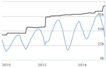
But oil, gas and coal prices are falling once again across March. The February bounce looks to have been a temporary phenomenon rather than the start of any structural recovery. The Brent curve is sliding again, with the front month contract falling back towards its January lows around 50 $/bbl. NBP and TTF curves are falling in sympathy, with prompt prices weakening into a mild spring. And ARA coal prices remain below 60 $/t and close to a nine year low as shown in Chart 1.

Chart 1: API2 2015 coal futures price chart

Source: Reuters

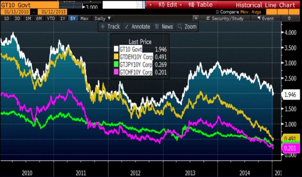
Generator fuel prices have also been buffeted by big moves in currency markets. While coal prices have fallen sharply in USD terms, this has been significantly offset by USD appreciation against the EUR. The USD has risen approximately 20% against the EUR since last September (about 10% against GBP).

The speed and scale of USD appreciation over the last six months is unprecedented over the last 30 years. It suggests a structural shift towards a stronger dollar as major European and Asian countries scale up monetary expansion in an attempt to fight economic weakness and deflation. Implied FX volatility has also increased sharply over this period, a red flag that it is prudent to place an increased focus on FX risk within energy portfolios.

Forward spread dynamics into 2015

While absolute commodity prices are of interest to generators, the primary driver of plant margins is relative moves across power, fuel and carbon prices. Charts 1 and 2 illustrate some interesting dynamics in the evolution of forward market implied gas and coal plant generation margins so far this year.

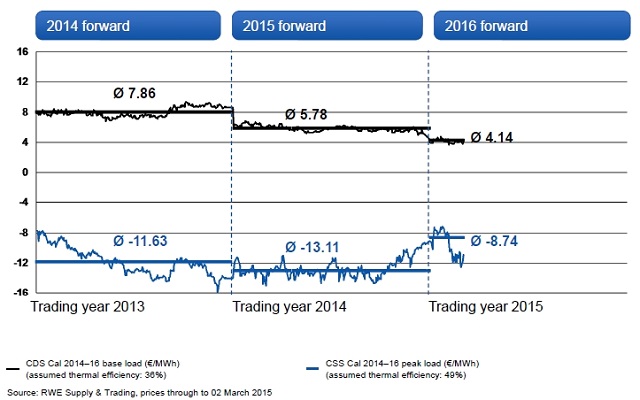
Chart 1: Germany clean dark and spark spreads

Source: RWE

German coal plant margins: As we have set out previously, coal plants dominate the setting of marginal prices in the German market. This explains the relative stability of German forward Clean Dark Spreads (CDS) in Chart 1. The gradual decline in forward spreads over the last three years reflects the increasing penetration of renewables as well as the commissioning of new and more efficient thermal capacity.

German CCGT margins: With coal plant setting marginal prices, the big decline in forward gas hub prices in Q4 2014 (as oil fell) has fed through into a significant bounce in Clean Spark Spreads (CSS), albeit still in deeply negative territory. Chart 1 shows the CSS recovery reversing somewhat across February. But the chart (using forward price data from Mar 2nd) does not show the subsequent increase in CSS over the last two weeks as gas prices have once again fallen.

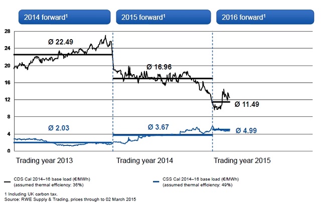
Chart 2: UK clean dark and spark spreads

Source: RWE

UK coal plant margins: The UK shows quite different margin dynamics given gas-fired plant dominate marginal price setting. Unlike in Germany, oil/gas price declines feed through directly into lower forward CDS as can be seen in Chart 2. This dynamic hints at tough times ahead for UK coal generators as they are faced by headwinds from both falling gas prices and an increasing carbon price floor (which will jump to 18 £/t in April).

UK CCGT margins: With CCGTs on the margin in the UK, CSS are relatively stable. The gradual recovery in gas-fired generation margins across the last 12 months reflects the tightening UK capacity balance. Although two mild winters (13/14 & 14/15) have helped to cap forward CSS recovery to date.

Overall the margin environment for gas and coal fired generators is still fairly bleak. However this is continuing to translate into capacity closures, good news for the margins of remaining generators. For example in the UK, Centrica and E.ON have recently announced their intentions to close CCGT plants after missing out in the first capacity auction. Weakness in forward CDS is also making life increasingly difficult for UK coal generators without capacity contracts. But commodity price movements may also have an impact on the relative value of gas versus coal plant.

Watch for gas vs. coal switching going forward

The last four years of commodity price evolution have firmly favoured coal plant margins over gas plants. Current market pricing still favours coal plants. But gas vs coal plant switching may yet become an important story in 2015.

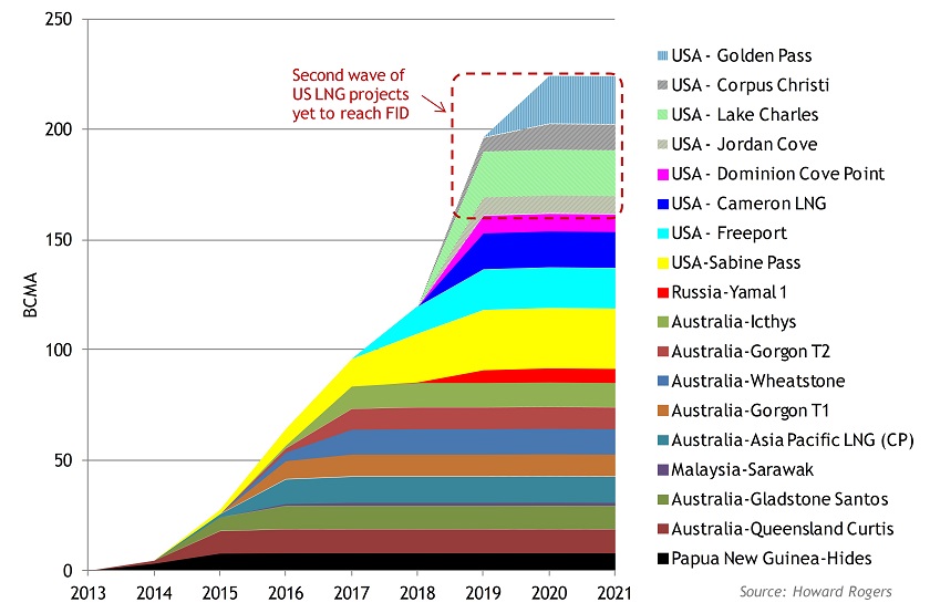
Global coal prices are now at levels where significant volumes of production are being curtailed. US coal producers look particularly vulnerable as the USD strengthens. This may act to stem further price declines even if global demand remains weak. Oversupply in the global gas market on the other hand is a relatively recent phenomenon. And rather than being curtailed, supply is ramping up substantially over the next 3 years (as we set out here).

The risk of further falls in European gas hub prices has been one of our key themes this year. These may act to close the gap between gas and coal plant competitiveness to the point that switching takes place again. The UK power market is the ‘canary in the coal mine’ for switching, given the penal impact of the carbon price floor on coal plant competitiveness. We will come back to analyse gas vs. coal switching dynamics in more detail soon.

The mountain of new LNG supply

Posted on March 16, 2015January 15, 2020 by David Duncan

Despite current conditions of oversupply, the LNG market is set to embark on a growth spurt over the next five years. The relatively long lead times for liquefaction terminal construction provide good visibility of supply volume growth towards 2020. And volume growth will be substantial even if it is only limited to projects already under construction.

More than 100 mtpa (138 bcma) of new LNG capacity is currently being built, half of this in Australia. More than 40 mtpa (55 bcma) of that volume is due to be commissioned by the end of 2016, across Australia, Malaysia, Indonesia and the first US export trains at Sabine Pass.

After several years of limited growth in new liquefaction capacity there is a mountain of new supply entering the LNG market. What is less clear is whether anticipated Asian demand growth will arrive in a timely fashion to absorb new supply.

Where is the new LNG coming from?

Chart 1 shows more than 150 bcma of liquefaction capacity that has reached Financial Investment Decision (FID) sign off and is set to be built by the end of the decade. The majority of this export volume will come from Australia and the US, both of whom are vying to substantially increase their presence as gas exporters. In addition, there is a ‘second wave’ of US export projects which are at an advanced planning stage but still awaiting FID sign off. If these volumes are included potential supply growth by the end of this decade swells to over 200 bcma.

Chart 1: A mountain of new supply over the next 5 years

(source Howard Rogers)

Australia vying for the heavy weight title

By the end of this decade Australia is set to overtake Qatar as the world’s largest LNG exporter. Projects under development can broadly be split into two groups:

Queensland: Three separate projects are being developed on Curtis Island (off the coast of Gladstone) to export coal seam methane (connecting the eastern Australian gas network to the global gas market).
Western Australia: The Chevron led Gorgon and Wheatstone LNG projects off the Pilbara Coast and the Japanese led Ichthys project in the Browse Basin will add to Australia’s existing WA based liquefaction capacity.

In total these projects account for almost 70 bcma of new gas exports under construction, the majority of which is scheduled to be delivered by 2018.

In theory Australia has the potential to grow its LNG exports further via the expansion of existing terminals as well as the development of new ones. But Australia has a cost problem given a strong currency, high labour costs and difficulty in accessing gas. It has become renowned as the most expensive place in the world to develop new LNG projects (e.g. 20-30% more expensive than the US & East Africa).

The recent decline in the Australian dollar may be starting to assist with this cost problem. But cost recovery on any new Australian export capacity will likely to require contract prices of at least 11 $/mmbtu for brownfield expansions, rising to in excess of $14/mmbtu for further greenfield projects.

The new waves of US export capacity

A first wave of about 50 mtpa (70 bcma) of US export capacity is under development for delivery by 2019. This consists of the first four trains at Sabine Pass, as well as the Freeport, Cameron and Dominion Cove projects, all of which have FERC approval and have secured long term capacity contracts.

However the current global oversupply environment may be exacerbated by the delivery of a ‘second wave’ of US liquefaction projects. This additional 50 mtpa of ‘second wave’ US projects are either contracted or covered under ‘heads of agreement’, but are yet to reach FID and commence construction. Until market conditions recover, this second wave of US projects are likely to face delays or even cancellation. However at current Henry Hub prices, this capacity does look to be the most competitive source of new LNG capacity beyond the projects currently under construction.

In the short to medium term, the project economics of other US export projects that are yet to find buyers looks to be very challenging indeed. Intrinsic margins from US exports to Asia and Europe have collapsed over the last 12 months, reducing the willingness of buyers to pay for capacity. Contract buyers are likely to be hard to find until crude prices recover and the current wave of new LNG supply has been absorbed.

Will the anticipated demand turn up?

New LNG supply volumes can be projected with relative confidence given liquefaction projects are already contracted and under construction. But there is much greater uncertainty over the timing and volume of anticipated growth in LNG demand. This opens up the possibility of a significant timing mismatch between new supply and demand which tips the global gas market out of balance.

New liquefaction capacity is being developed against a backdrop of a structural increase in global gas demand, particularly in Asia. However a significant volume of new LNG is being contracted by portfolio players, rather than on a destination specific end-user basis. In addition, a number of higher growth importing nations (e.g. China and India) have relatively low long term contract levels.

The greatest demand side uncertainty sits with China. Over the last 12 months, China has been dampening industry expectations around its much anticipated increase in LNG demand. This is consistent with the signing of 68 bcma of framework agreements for pipeline imports from Russia. But the ongoing development of Chinese regas capacity is setting up the option for significant growth in LNG imports at the right price.

More broadly, Asian LNG demand is also vulnerable to a weakening global economic growth outlook and the prospect of Japanese nuclear restarts. Falling LNG prices may induce some demand response, particularly from more opportunistic buyers such as China. But when committed new supply is overlaid on a weakening demand outlook, the global gas market looks to be heading into a period of pronounced oversupply towards 2020.

Monetising the value of flexible gas & power assets

Posted on March 9, 2015January 15, 2020 by David Duncan

Flexibility value is a term often loosely used in association with gas and power asset optionality. It is a simple and widely accepted principle that asset flexibility has an associated value. But the practicalities of quantifying and monetising this flexibility value are often more complex.

Flexibility value has become much more important in European gas and power markets over the last few years. This is because of an increasing prevalence of assets with ‘at the money’ and ‘out of the money’ optionality.

For example most European gas-fired power plants have a variable cost at or above wholesale power price levels. Gas storage capacity has ‘at the money’ value characteristics given the weakness in seasonal hub price spreads. Similar logic applies for LNG supply contract diversion rights given regional spot price convergence.

Quantifying and extracting the value of asset optionality depends on the monetisation strategy adopted by the asset owner or investor. There are a range of monetisation strategies that are commonly applied which are distinguished by level of sophistication and risk/reward trade off. These include passive contracting strategies as well as more dynamic hedging and optimisation strategies.

In this article, the first in a series on value monetisation, we summarise five common strategies applied to the monetisation of flexible assets, using practical examples as an illustration. Then in subsequent articles we will undertake a comparison of the pros and cons of each of these strategies. We will also explore practical considerations in developing an appropriate monetisation strategy for a specific asset or portfolio.

Five ways to skin a cat

The five most common strategies for hedging and optimising flexible assets are summarised in the table below, followed by a summary description of each. We use the term ‘assets’ in a broader sense to capture physical infrastructure as well as contracts. Some of these strategies are more commonly applied than others given more palatable risk/reward characteristics. However we describe a full spectrum of strategies to highlight contrasting approaches.

Strategy	Description
1. Spot optimisation:	Intrinsic & extrinsic value managed against spot prices
2. Static Intrinsic:	One off intrinsic hedge (& matching asset dispatch)
3. Static Intrinsic + Extrinsic:	Sale/contracting of intrinsic + extrinsic value
4. Rolling intrinsic:	Rolling adjustments to intrinsic hedge (when profitable)
5. Delta Hedging	Dynamic hedging of exposures in response to price changes

Chart 1 then illustrates a stylised comparison of risk/reward tradeoffs across the five different strategies (something we will revisit in more detail in the next article in this series).

Chart 1: Value frequency distributions for the 5 strategies (source Timera Energy)

1. Spot optimisation

In many ways the purest asset monetisation strategy is optimisation of an asset against current and expected future spot price levels. Under this strategy no forward hedging is undertaken. The advantage of this is that there are no associated hedging costs. The disadvantage is the strategy results in a relatively wide distribution of asset returns (i.e. higher earnings risk).

This strategy is often implemented out of necessity rather than choice. This is the case for ‘out of the money’ assets e.g. gas peaking plant or for assets with a high proportion of extrinsic value e.g. very fast cycle storage assets. In both cases, hedging beyond the prompt period (i.e. close to dispatch) is difficult.

Implementation of a spot optimisation strategy requires a strong stochastic asset modelling capability to analyse price behaviour and decisions on exercise of asset optionality. This is particularly the case with assets which have more complex inter-temporal flexibility (e.g. gas swing / storage). In addition a capable prompt trading function and associated supporting functions, systems and processes are required.

A pure spot optimisation strategy represents one extreme of the value monetisation spectrum. But in practice, spot optimisation is usually matched with some form of forward hedging where possible.

2. Static Intrinsic

The other end of the value monetisation spectrum is represented by the static intrinsic strategy. This is a simple strategy where the asset is optimised and hedged on a ‘one off’ basis. This strategy is focused on locking in intrinsic value. It does not allow capture of extrinsic value and is subject to market timing risk. The strategy is therefore limited in its application.

The advantage of a static intrinsic strategy is that it requires very little commercial organisation capability beyond a basic operational support function and back office. It also has a relatively low associated earnings risk (e.g. residual availability and credit risk). This strategy was historically applied in the classic project finance structures for early independent power projects, read this post here for you to know what strategy and other stuff about your funds and how you finance your business. It is still occasionally used for ‘deep in the money’ assets with little extrinsic value.

However the management of intrinsic asset value is typically accompanied by some form of static or dynamic strategy to facilitate the capture of extrinsic value.

3. Static intrinsic + extrinsic

This strategy is a variation of the static intrinsic approach, but one which enables up front monetisation of asset extrinsic value. This is achieved by selling asset optionality to a third party (assuming a buyer can be found). The strategy can be executed on a one off basis e.g. signing a long term tolling contract on a CCGT asset, or as a series of contracts e.g. a storage asset owner selling capacity contracts of different durations/configurations on a single asset.

The strategy can be implemented either on a physical contract basis or using ‘virtual’ or ‘synthetic’ deals. It may also be adopted in response to a regulatory requirement where asset Third Party Access (TPA) is mandated e.g. for gas transportation capacity and some storage assets.

The strategy is attractive in that there is generally a relatively low residual earnings risk over the horizon for which the asset is contracted. Although residual risk may increase with more dynamic capacity sales strategies, e.g. depending on contract timing and the degree to which the owner retains market risk.

This strategy is very common for more risk averse asset owners such as independent producers or smaller portfolio players. Implementation requires a commercial support capability (e.g. sales strategy / product development). But importantly it does not require a trading capability (and associated cost/complexity). Given the costs and risks of extrinsic value monetisation sit with the contract counterparty, the asset owner will often incur a substantial value discount.

4. Rolling Intrinsic

Probably the most common strategy adopted for monetisation of flexibility value is the rolling intrinsic strategy. Asset flexibility is optimised & hedged against the forward curve, with the owner ‘rolling’ or adjusting hedges if better opportunities present themselves. In other words re-optimisation and hedge adjustment is only undertaken if profitable (i.e. adjustments are risk free). Most importantly it enables the capture of some extrinsic value on an ongoing (rather than a one off) basis.

The owner does not retain any downside market risk as the intrinsic hedges are only unwound if profitable adjustments can be made to the strategy. This reduces the market timing risk problem associated with the static strategies (2 & 3). But it means that the asset owner retains some earnings variability, given access to upside is a function of market price dynamics.

A rolling intrinsic strategy requires an active trading capability. But it does not require sophisticated dispatch and hedge modelling. The strategy represents a practical way of extracting extrinsic value while limiting downside earnings risk. As a result it is a very common strategy employed to monetise value of power, gas and LNG assets. This is particularly the case in illiquid markets where significant transaction costs can be cleanly accounted for when identifying profitable adjustments.

5. Delta hedging

The delta hedging strategy is a more sophisticated approach for the dynamic hedging of asset optionality. Asset flexibility is optimised against current & expected future spot prices as for the spot optimisation strategy (1.). But in this case, probabilistic forward ‘delta’ exposures are also calculated and hedged using linear products (i.e. fixed price/volume futures or forwards) in the underlying market.

The delta hedging strategy can be described using a simple CCGT example. Asset dispatch is optimised against spot power, gas and carbon prices (e.g. via the day-ahead or within-day markets). But in addition a probabilistic calculation of forward ‘delta’ sparkspread exposures is undertaken across the time buckets of available traded contracts. This is typically deconstructed into the gas, power and carbon legs that can be liquidly traded. The forward delta exposures are then hedged and hedges are dynamically adjusted as deltas change with market price movements.

The benefit of a delta hedging strategy is that it targets capture of the ‘full’ option value of an asset, whilst reducing earnings risk when compared to a spot optimisation strategy. But the owner still retains exposure to downside market risk as asset exposures are not fully hedged until delivery.

Trading desks often favour this strategy as it creates:

Liquidity – by generating a requirement to dynamically adjust hedges in the market
Cash – given hedge adjustments involve buying the underlying at lower prices and selling them back at higher prices (monetising volatility)

However, successful delta hedging requires a capable and experienced trading function and a sophisticated analytical capability (e.g. to calculate forward delta exposures). It is also not suited to all assets in all market conditions. Delta hedging requires relatively stable delta exposures and reliable market liquidity. But most importantly, theoretical or modelled value can be killed by market transaction costs. This means the successful implementation of delta hedging requires the combination of sophisticated but practical commercial and analytical expertise.

Comparing strategies

In our next article in this series we come back and undertake a more detailed comparison of the pros, cons and pitfalls associated with these five strategies. Strategy application is typically a case of ‘horses for courses’. No one strategy is best and in many cases the actual monetisation strategy adopted may be a combination of several strategies, particularly in the case where the asset sits within an integrated portfolio. This means it is important to pro-actively develop a monetisation strategy that is tailored to the risk/return tolerance and organisational capabilities of the asset owner.

Power capacity payments are coming across Europe

Posted on March 2, 2015January 15, 2020 by David Duncan

European power markets are slowly but steadily moving towards implementing capacity remuneration mechanisms for flexible generation. A consistent pan-European solution for capacity remuneration looks unlikely. Instead the approach and pace of implementation is being driven by security of supply concerns in individual countries. However a regulatory consensus is emerging as to the need for some form of remuneration for flexible capacity as renewable generation volumes rise.

Theoretical discussions are raging across Europe as to the ‘missing money’ problem of under remuneration of peaking capacity, the academic basis for capacity payment intervention. But ultimately capacity remuneration implementation is likely to be driven by practical rather than academic considerations.

In the absence of capacity payments (or much higher power price volatility), renewable capacity subsidisation across Europe will squeeze flexible generator margins to the point that assets close. The current capacity oversupply situation across much of Europe may provide a temporary buffer, but ultimately plant closures will undermine security of supply.

Different approaches across Europe

Capacity payments in power markets are not a new concept. Several markets in the US have implemented capacity markets with varying degrees of success. There are also European markets that have some form of capacity payments e.g. Ireland and Spain. But for the larger North West European power markets, the design & implementation of capacity payment mechanisms is a relatively new step.

There are broadly three forms of capacity remuneration model being considered:

Central buyer solution: for example as has been implemented in the UK in 2014 (for capacity delivery in 2018/19), driven by security of supply concerns over a rapidly tightening system capacity margin.
Supplier obligation solution: for example as is being implemented in France in 2015 (for 2016/17), driven by concerns over capacity to meet peak winter heating load.
Strategic reserve payments: for example the ‘Strategic Generation Reserve’ contracts that have been awarded in Belgium in the lead up to the current winter to address system tightness concerns after nuclear outages.

Chart 1 provides a summary of the approach to capacity payments across Europe.

Chart 1: Capacity remuneration across Europe

Source: EY

Strategic reserve payments are being used as a convenient temporary (or ‘stepping stone’) solution to address system capacity issues. There is typically a lower regulatory hurdle for introducing these payments compared to transitioning to a more structural capacity market solution. The payments are being introduced under the guise of greater powers for the system operator to contract reserve. But there is increasing disquiet within the industry as to the lack of transparency around remunerating capacity in this way.

For example, the UK Supplemental Balancing Reserve (SBR) payments are being used as a somewhat opaque ‘stop gap’ means of remunerating capacity over winter periods, while the more structural capacity market solution is rolled out. Germany has taken a different but equally controversial approach by mandating certain assets of strategic system importance remain open for reserve purposes.

Oversupply in Continental power markets has reduced the immediate urgency for structural capacity remuneration solutions. But as time passes, increasing renewable output will only further compromise the economics of flexible peaking assets. It is unlikely that politicians and regulators will be willing to stomach the power price volatility required to keep adequate peaking capacity on the system. And local transmission constraint issues (e.g. in markets like Germany) are also pressuring regulators to respond.

A number of countries across Europe are now openly considering more structural capacity remuneration solutions e.g. Germany, Belgium, Poland and Italy. The momentum for capacity remuneration is only likely to increase over time with interesting implications for asset margins and investment returns.

Commercial lessons learned from UK capacity market implementation

The UK led the way in Europe with implementation of traded wholesale gas and power markets. This was driven primarily by a pro-liberalisation regulatory agenda. The UK again finds itself leading the way with the design and implementation of a capacity market. But this time it is driven more by reactive necessity than proactive ideology. The UK is facing a rapid decline in system capacity margin, at the same time growth in renewable output threatens to close a number of thermal assets required to provide peaking capacity.

The UK capacity market implementation is not a shining example of how to design and deliver capacity support from a policy perspective. But the commercial ‘lessons learned’ by UK generators in the lead up to the first auction have a broader relevance for generators across Continental power markets as they prepare for capacity payment mechanisms.

The transition to capacity remuneration may in some ways appear to be a relatively minor tweak to market design. But in practice capacity payments have an important structural impact on thermal asset risk/return profiles and generation portfolio dynamics. The following are some higher level observations on the transition to capacity payment support:

Capacity vs energy circularity

Capacity payments add a more stable margin stream for flexible thermal assets. But they tend to have an important adverse impact on wholesale energy margin by supporting higher levels of system capacity. This tends to increase competition to provide the marginal MW of capacity and therefor reduce energy market rents. Analysis of the interdependence between capacity and energy pricing and the associated impact on generation margins, provides an important foundation from which to understand the commercial impact of capacity payments.

Investment, technology and costs

As capacity constraints begin to bind, the cheapest source of incremental flexible capacity will typically be provided by keeping open existing thermal plants that have a competitive fixed cost structure and that have capital costs which are already paid down (e.g. less efficient CCGTs). Capacity payment support can fundamentally change the economics of these assets (most of which are currently cash flow negative).

Once existing capacity options are exhausted it is important to understand the economics of new build options. Capacity payment mechanisms may skew new build investment economics. Capacity payments tend to favour lower capex small scale peakers (e.g. diesel generators, reciprocating engines and small gas turbines) ahead of more efficient but more capital intensive technologies (e.g. new CCGTs).

Capacity payments also impact the financing opportunities for new plants. A consensus is emerging across lending banks that debt sizing should be based on the capacity payment margin stream, with equity required to support the balance of the investment.

Capacity pricing dynamics

There are some good benchmarks for capacity pricing that can be derived from a combination of technology costs and historical price data from existing capacity markets. Conclusions on capacity pricing bounds can be drawn to some extent independently of the capacity mechanism design. For example:

Lower price bound: A reasonable lower bound benchmark for the capacity prices (in a market that faces a capacity constraint) is provided by the fixed costs of thermal peaking assets that would otherwise close (e.g. less efficient CCGTs).
Upper price bound: Reasonable upper bound benchmarks can be derived from the costs of delivering incremental new flexible capacity. It is important to note however that capacity mechanism design may skew this benchmark towards lower capex smaller scale peaking assets rather than CCGT.

Asset lifetime horizon

Perhaps the most important conclusion from preparations for the UK capacity market is to develop a strategy for capacity remuneration over an asset lifetime horizon. It is human nature to focus on the most immediate problems to hand. In the case of capacity payments this can mean focusing on capacity returns over a near term horizon e.g. defining a specific bidding strategy for the next capacity auction. But it is much more important to develop generation portfolio and investment strategies around the interdependent evolution of wholesale energy and capacity margin streams over a longer term horizon. This means deriving capacity bids based on a risk adjusted asset lifetime ‘Net Present Value’ view.

It is easy to ignore capacity remuneration until there is greater certainty around policy design and implementation. But the UK capacity market experience suggests that the specifics of policy design do not preclude generators from taking proactive steps to alter their investment and generation portfolio strategies. In fact there is a clear first mover advantage from anticipating the structural impacts of capacity payments on asset margins, portfolio structure and investment strategy.

European hub prices under pressure in 2015

Posted on February 23, 2015January 15, 2020 by David Duncan

After several years of relative stability, the European gas market has entered a more dynamic transition phase. Spot prices at European hubs have faced strong downward pressure since summer last year. The threat of Russian supply disruptions provided some temporary support for forward prices in advance of the current winter. But hub price declines have extended along the NBP and TTF curves into 2015.

There are two main factors driving spot and forward price declines:

A reduction in oil-indexed contract prices due to the recent slump in oil prices
Surplus flows of LNG cargoes into Europe due to weak Asian spot prices

Overlaying the fact that European gas demand has been relatively weak given a mild winter and it appears that hub prices have held up surprisingly well in Q1.

Prices have been supported in Q1 by oil-indexed supply contract volume profiling. But as 2015 progresses, this effect is set to reverse, causing renewed downward price pressure on hub prices into the summer.

Hub price drivers into 2015

The sharp oil price declines of Q4 2014 & Q1 2015 are yet to fully flow through into long term oil-indexed contract prices. That means contract prices are currently significantly higher than hub prices. Most contracts have a six month indexation lag to oil, which provides good forward visibility of a sharp fall in contract prices in Q2 & Q3 2015 (towards 6-7 $/mmbtu). The blue range in Chart 1 illustrates the downward move in contract prices as 2015 progresses relative to NBP forward prices in green.

Chart 1: European gas pricing in a global context

Source: Timera Energy

The current premium of contract over hub prices provides a strong incentive for contract buyers to profile their annual contract take. Volume take in many contracts is currently being minimised in Q1 (given hub gas is cheaper) in anticipation of higher contract volume take at lower oil-indexed prices across the remainder of the year (once price lags feed through fully).

Volume profile optimisation varies by supply contract. While European pipeline contracts broadly have a uniform structure (e.g. annual take or pay, daily swing constraints, oil products indexation), the pricing and volume terms of individual contracts vary significantly. But while specific volume take incentives may vary across contracts, the rapid decline in oil prices has caused a sharp reduction in pipeline gas flow into Europe across Q1 to date (in the order of a 40% y-o-y reduction in Russian volumes in Jan 15).

Reduced volumes of pipeline contract supply are currently being offset to some extent by:

Higher storage withdrawal volumes (a temporary effect over the Q1 withdrawal season – see Chart 2)
Higher flows of flexible LNG supply into European hubs (as we set out last week)

But the scale of contract volume profiling is definitely a factor currently supporting spot prices.

Chart 2: European aggregate storage inventories

Source: Gas Infrastructure Europe

Renewed downward pressure as the year progresses

After sitting at a premium to hub prices for most of the last decade, long term contract proxy price benchmarks have actually fallen below forward hub prices for the majority of 2015 (the blue range crossing over the green line in Chart 1). This suggests the contract volume profiling dynamics described above will reverse as 2015 progresses.

Once contract prices fall below hub prices, contract buyers have the incentive to maximise contract volume take, selling any surplus gas at the hubs to secure a premium. It is this arbitrage dynamic that acts as a strong force to maintain hub prices within a range of oil-indexed contract prices. But as the year progresses, contract prices are set to swing from being a source of hub price support in Q1, to a significant drag on prices across Q2 and Q3.

There are a couple of factors that may provide some hub price support as the year evolves. The potential for earthquake related reductions in production at the large Groningen field in the Netherlands were announced last week. But the volumes are relatively small compared to the scale of pipeline contract and LNG import volumes. The Groningen reduction (still subject to political debate) is in the order of 5 bcm reduction (less than 1% of European gas demand).

In addition supply contract negotiations over recent years (e.g. with Gazprom) have resulted in increased annual take or pay constraint flexibility. This means that contract owners have a greater ability to reduce gas volume take during periods of oversupply.

But the big incremental pressure on European hubs in 2015 may come from the LNG market. Hub prices are facing additional pressure from falling Asian spot & long term contract LNG prices (the red lines in Chart 1). Lower Asian LNG prices make Europe a more attractive market for flexible LNG supply volumes. The flow of surplus LNG cargoes into Europe is likely to build into the summer as a result of:

The seasonal reduction in Asian LNG demand (the pronounced seasonal spot price shape can be seen over previous summers in Chart 1)
The ramp up in new liquefaction capacity as projects come online (in Australia, Indonesia and Colombia)

The combination of pipeline contract profiling and surplus LNG cargoes suggests to us that the risk around European hub prices is firmly to the downside as 2015 progresses.

Europe is now the hub of the global gas market

Posted on February 16, 2015January 16, 2020 by David Duncan

In the three years following the Fukushima crisis, LNG supply played a relatively limited role in influencing European hub prices. Flexible LNG supply volumes flowed away from Europe to Asia, with Asian LNG spot prices providing the key global spot price signal.

These dynamics have changed in quite dramatic fashion since the summer of 2014. Asian spot LNG prices have declined rapidly to converge with European hub prices at around 7 $/mmbtu. As the global LNG market tips into a state of oversupply, surplus LNG cargoes are flowing back into Europe and European hub prices are acting as a key global price support.

LNG market oversupply

Q2 2014 marked the start of a new phase in global gas pricing. As a warning sign, Asian spot LNG prices halved across the first half of 2014, from 20 to just above 10 $/mmbtu as illustrated in Chart 1. This was exacerbated by a lack of underground gas storage and limited tank storage in Asian LNG importing countries.

Chart 1: Asian spot LNG vs European and US hub prices

Source: Reuters

European hub prices slumped in sympathy. This was driven partly by surplus LNG flowing back into Europe, but also by the withdrawal of high European storage inventories given the loss of 57 bcma of demand (y-o-y) as a result of a mild winter. LNG spot prices made a brief recovery in Q3 in anticipation of winter. But as confirmation that a structural transition was taking place, spot prices continued their decline into the winter of 2014-15, with the crude price slump and a surplus of spot LNG cargoes adding to downward price pressure. Last week Asian spot prices slumped below European hub prices with buying interest in Asia having dried up.

Price declines have not been limited to the spot market. Oil-indexed Asian contract prices are also set to fall towards 7 $/mmbtu this summer as the lagged impact of the crude price fall feeds through into contract price formulas. This means that the structural Asian price premium over European hubs has essentially disappeared. The global market looks to be entering a new phase of lower and more convergent regional gas prices.

The role of Europe in an oversupplied global market

LNG market oversupply may be a temporary effect due to a mismatch between the timing of global demand growth and new supply. But it is also possible that the global gas market may be entering a more structural phase of oversupply lasting a number of years. The nature of this period of oversupply will have important implications for global LNG and European hub prices.

In order to makes sense of the commercial impacts of an oversupplied world it is important to have an analytical framework from which to understand global gas pricing dynamics. The foundation of such a framework can be built on a depiction of the global gas market as three separate regional markets, each cleared by a regional spot market:

The US – cleared by Henry Hub spot prices
Europe – cleared by spot prices at European hubs
Asia – cleared by spot LNG prices

Flexible LNG supply sources are then the key mechanism which clears the global market across the three regions. Flexible LNG supply consists primarily of divertible LNG contracts, uncontracted LNG production and US exports (from 2016). This often comes in the form of flexibility to move gas within the portfolios of larger energy companies which have broad LNG supply chain exposures (e.g. BG, Shell, Chevron, Exxon).

During the post Fukushima phase of market tightness, flexible LNG supply volumes flowed away from Europe to Asia, driven by a significant Asian spot price premium. Now in an oversupplied global market, flexible LNG is flowing back into European hubs. Europe’s ability to soak up surplus flexible LNG volumes is set to be the key driver of pricing dynamics through the period of global oversupply.

Chart 2 illustrates the projected European versus global LNG market balance in 2016. The left hand section of the diagram shows the supply and demand balance for the European gas market. The right hand side shows the global LNG market balance. In the current oversupplied world, European hubs need to absorb surplus LNG supply. In practice this means LNG flows displace flexible Russian gas volumes (e.g. swing contract volumes above take or pay).

Chart 2: Projected European vs global LNG balance in 2016

Source: Timera Energy

But at the point that the volume of surplus LNG flowing into Europe exceeds flexible pipeline supply volumes, European hub prices may need to fall substantially in order to clear the market. Practically this would likely be achieved by a combination of:

Reduced Russian pipeline exports to Europe (e.g. negotiated take or pay concessions)
Gas displacing coal in the European power sector (important for CCGT margin recovery)
A reduction of US LNG exports if European hub prices do not cover variable export costs (once US export flows come to market in 2016)

Europe’s ability to soak up surplus flexible LNG volumes will become an important driver of global pricing dynamics through the current period of global oversupply. In turn LNG flows are set to become a key driver of European hub pricing dynamics. The volume of LNG flow into Europe will influence absolute hub price levels. The profiling of flow patterns will also impact summer/winter hub price spreads and price volatility. Across the space of the last six months, the evolution of the global LNG market has rapidly taken centre stage as a future driver of the European gas market.

This week’s article was co-authored by Howard Rogers, a Senior Advisor with Timera Energy and Director of Natural Gas Research at the Oxford Institute for Energy Studies.

Market benchmark for gas flexibility value

Posted on February 9, 2015January 15, 2020 by David Duncan

After a recovery in the first half of 2014, seasonal price spreads at European hubs have again fallen back towards historically low levels (currently around 1.70 €/MWh). Given summer/winter spreads are the key market price signal for seasonal flexibility, there has been an associated decline in the market value for storage capacity.

GasTerra has been auctioning storage capacity for 4 years now. The standard bundled unit (SBU) has become a transparent and objective benchmark for the value of flexibility in the NW European gas market. It also provides a useful benchmark for the level of extrinsic value which capacity buyers are prepared to pay for, over and above the intrinsic spread value that can be hedged against forward prices.

The latest auction for GasTerra capacity was held last week. In this article we show some simple analysis of the results and consider implications for flex value.

Seasonal spread evolution

Chart 1 shows the evolution of seasonal spreads at the Dutch TTF hub since 2008. It clearly illustrates how the development of an oversupply of seasonal flexibility has driven down summer/winter spreads. Spreads have fallen from above 6 €/MWh in 2008-09 to below 2 €/MWh in 2013-14.

Chart 1: Evolution of Front Year TTF summer winter spreads

Source: Timera Energy

There have been isolated years where spreads have made a brief within year recovery. For example high volumes of storage withdrawals in Q1 2014 after a mild winter, saw a sharp drop in summer prices which temporarily fed through into a higher summer/winter spread. But as yet there is no evidence of any structural recovery in seasonal spreads that can be observed in forward market pricing.

Feb 15 GasTerra auction result

Hub price signals are now the primary driver of the value of European gas flex (e.g. storage, swing). Seasonal hub price spreads drive the return on seasonal response. Prompt volatility drives the return on rapid flexibility response.

The auction clearing prices for GasTerra SBU capacity (shown in Chart 2) illustrate the strong relationship between seasonal storage capacity value and TTF summer/winter price spreads.

Chart 2: Evolution of GasTerra SBU auction clearing prices

Source: ICE/GasTerra

Over the last 4 auctions (Q4 2013 to Q1 2015) prices for GasTerra capacity have stabilised in a 2-3 €/MWh range. The different results across these auctions can be explained by marginal differences in forward spreads, absolute gas price levels and extrinsic (volatility) value capture dynamics.

We have undertaken a simple analysis of the outcome of the February 2015 auction in Chart 3. In order to do this we have calculated our view of the expected value of the GasTerra SBU using the Timera Energy storage modelling suite (shown on the left). This is then compared to the actual auction results (on the right).

There is a relatively high proportion of extrinsic value given that seasonal spread levels are so low (i.e. storage optionality is close to ‘at the money’). Our analysis indicates that the market is paying for just over 60% of extrinsic value. This is consistent with the logic that capacity buyers need to allow for a margin to cover trading costs (e.g. risk capital and transactions costs).

Chart 3: Feb 2015 GasTerra auction result analysis

Source: Timera Energy

Some practical implications for storage capacity

There is a soft lower bound on seasonal spreads at around the 1 €/MWh level reflecting the transactions costs involved in cycling storage capacity to move gas from summer to winter. Market pricing is pretty close to that level with current spread levels around 1.70 €/MWh. That means that there is asymmetric upside from spread recovery.

However asymmetric upside does not in its self mean that spreads will necessarily recover anytime soon. But it does impact the management of exposures by capacity owners and buyers. For example it is being reflected in the behaviour of storage operators (e.g. GasTerra, TAQA Bergermeer) who are selling capacity on an indexed basis (i.e. retaining spread exposure when they sell capacity).

There are going to be several important factors to watch moving into 2015 that could impact the evolution of European seasonal hub price spreads:

The seasonal volume profile of LNG flows into Europe (e.g. high volumes in summer given weaker global demand, lower volumes in winter given stronger global demand)
The gas vs coal plant competitive balance and its impact on power sector gas burn (particularly in the UK with the carbon price floor)
The impact of weakening economic growth projections in Europe and associated impact on gas demand

We will keep a close eye on these factors as the year evolves.

Brent curve collapse in animation

Posted on February 2, 2015January 15, 2020 by David Duncan

The Brent crude forward curve had a wild ride across 2008 and 2009. The commodity supercycle peak dragged spot crude towards 150 $/bbl, with forward prices following almost in parallel. Then the financial crisis saw spot prices crash and a deep contango open up along the curve. But since 2010, crude prices have moved in a tighter range accompanied by a relatively flat and stable forward curve. That is until Q4 2014.

The wild ride is back again. As the crude market has taken on board the reality of shorter term oversupply, spot prices have slumped in a similar fashion to 2008. A steep contango has again opened up along the curve reflecting a pronounced near term supply glut.

Last week we set out two important benchmarks that are influencing crude price behaviour via the marginal cost dynamics of US shale oil production:

Spot prices may need to breach the SRMC of US shale (~40 $/bbl) to curtail production and stabilise the market.
The curve may need to sit below the LRMC of US shale (70-80 $/bbl) to curtail investment in new US shale wells.

In today’s article we use an animation of the evolution of the Brent forward curve to illustrate how these benchmarks relate to spot vs curve behaviour. We also look at a third important benchmark driving oil curve dynamics: the contango driven physical storage arbitrage.

Brent in animation

Chart 1 shows a monthly time step animation of the evolution of the front 5 years of the Brent curve since 2008 (note the animation may not work in some older web browsers). This follows on from a similar animated analysis we did previously of UK NBP gas curve evolution.

Chart 1: Evolution of Brent crude spot and forward prices

Source: Timera Energy (based on ICE Brent Futures settlement prices)

The chart illustrates some interesting characteristics of crude curve behaviour:

2008-09: A period of major market transition with the commodity supercycle peak followed by the financial crisis crash and then a relatively sharp recovery. There was a strong parallel curve shift during the move up towards 150 $/bbl. This then gave way to a spot price slump to 40 $/bbl. However the tail of the curve held up at around 70 $/bbl (similar to the current Brent curve).
2010-14: Both spot prices and the curve recovered into 2010 as the demand shock from the financial crisis eased. Across this period crude moved in a tighter $90-120 range. The tail of the curve was anchored between $90-100 (which led to curve backwardation in periods of tighter spot prices). A market consensus developed across this period that there was an $80-90 floor in crude prices driven by LRMC of unconventional oil production.
Q4 2014+: A strong market consensus rarely bodes well for price stability. The spot and curve price decline since Q4 2014 has so far followed a similar path to the 2008 slump. However the sharp recovery bounce seen in 2008 is unlikely to be repeated this time given the time required for supply side response to impact prices, as we described last week. As in 2008, a pronounced curve contango has again opened up.

Contago is back

Physical storage arbitrage is an important driver of crude curve dynamics. Curve contango means that oil can be bought at today’s spot price, stored in tanks or on anchored vessels and sold forward at higher prices. The contango price spread is locked in subject to delivery of the stored oil. A recent pickup in interest for US storage capacity and the chartering of tankers for floating storage plays illustrates the market reaction to the widening crude curve contango.

It is interesting to contrast physical arbitrage in the crude market with the LNG market. While there are genuine arbitrage opportunities available to the owners of seasonal gas storage capacity, the LNG market is more complicated. Much pain has been suffered over the last year on attempted intertemporal LNG price spread plays. A number of portfolio players purchased what appeared to be cheap LNG cargoes last summer (around 10-11 $/mmbtu) with a view to selling them into higher Asian winter prices. But the buyers retained seasonal price spread risk, given an inability to sell the cargoes forward (because of liquidity constraints). This has left buyers exposed as LNG spot prices have now plunged well below the price levels from last summer (currently trading around 7 $/mmbtu).

During the 2008 crude price slump, the 12 month contango opened up to 20 $/bbl and storage arbitrage provided a key source of spot price support. The current Brent and WTI curve 12 month contangos are ranging around the 10 $/bbl mark. Not yet as pronounced as 2008, but still presenting an attractive arbitrage opportunity subject to storage capacity access. As the fallout from the current decline in oil prices continues, storage arbitrage will act as an important force supporting spot prices and pulling down forward prices.

Crude impact on gas pricing

This article concludes our three part series on crude pricing dynamics. While we have explored forward curve dynamics in today’s article it is spot oil prices that have the most important impact on gas and LNG prices. European long term gas contract prices are predominantly linked to oil product spot prices (which trade at a basis to spot crude), typically with a six month time lag. Asian LNG contracts are indexed to crude, often with a shorter time lag.

So it is possible to predict today within a reasonable margin of error the level of European and Asian gas contract prices coming out of spring and into summer. And those levels are substantially below current contract price levels. As a result there is going to be heavy downward pressure on European hub prices from cheaper pipeline contract gas and an increased flow of cheap flexible LNG back into Europe. Add the potential for rapid withdrawal from well stocked gas storage facilities and there may be a wild ride to follow in the European gas market in 2015, a theme we will return to in subsequent articles over the next few months.

Supply side response to lower crude

Posted on January 26, 2015January 15, 2020 by David Duncan

This is the second article in a three part series on falling crude prices. In the first two of these articles we look at the two key factors behind the current price decline:

A weakening global demand outlook, with global economic growth expectations weakening. Specifically in some of the larger oil importing countries (e.g. Japan, China and India)
A surge in production, driven predominantly by the expansion of US shale oil production but also by robust production from some of the larger conventional producers (e.g. Libya and Iraq)

Last week we focused on weakening demand. But the demand side provides limited insight into the shorter term drives of crude market price dynamics. Demand for oil is not particularly timely in its price responsiveness. So it is likely to be supply side response that determines when and at what price level the crude market stabilises. That is the focus of today’s article. Some of the material in this article draws on useful recent analysis on production dynamics by Goldman Sachs.

Producer strategy

Analysis of the oil market has historically been clouded by the cartel behaviour of OPEC producers. But the relevance of OPEC’s price/volume strategies has been eroded by the surge in US shale production. Growth in US shale output has been a big factor behind the current oversupply. But the economics of shale production are also likely to drive the marginal pricing dynamics that stabilise the crude market.

Several conspiracy theories have been floated on collusive behaviour that has contributed to the decline. For example OPEC is happy to see US and producers suffer at lower prices or Saudi Arabia and the US are acting to hurt Russian interests.

But the reality is that OPEC (and Saudi Arabia) has limited power to act to stem the current price rout. All producers are suffering together from lower oil prices. Not a single OPEC member can balance their budget at current oil price levels as shown in Chart 1 via an interesting graphic published in the Economist.

Chart 1: Budget impact of the crude price slump

Source: The Economist

The traditional assumption has been that OPEC producers will respond to price declines by cutting production volumes. But the reality in the current world of falling prices is that producers are incentivised to increase production because they need the revenue. They are not incentivised to cut production to boost prices. This removes the focus on OPEC production volume dynamics and shifts it to the economics of US shale oil producers who dominate the marginal section of the crude supply curve.

How will supply respond?

In order to address the current oversupply in the crude market, prices need to fall to a level that curtails production. There are two important benchmarks here:

Short run marginal cost (SRMC): Producers will scale back production if they cannot cover their operating cash costs at current price levels (subject to the influence of protection from existing hedge positions).
Long run marginal cost (LRMC): New production will not be commissioned if prices do not cover life cycle investment costs (note: this is driven more by prices over an investment horizon than the current spot price, albeit it with an obvious linkage).

In conditions of plentiful supply, spot price movements in commodity markets tend to be focused more on SRMC than LRMC dynamics. There is usually a rapid supply curtailment response if producers cannot cover variable costs. With cash operating costs of around 40 $/bbl, the more marginal US shale plays may act as important price support in the short term (caveat the risk of prices overshooting to the downside before there is an adequate production response).

However Goldmans’ argument is that the LRMC dynamics of US shale will also be a key driver of short to medium term production response. This is a function of the scalability of shale production and short production lead times. A high decline rate on new wells means that there is a relatively fast investment replacement cycle. In other words the life cycle costs of shale wells (at 75-80 $/bbl) play a much more important role in influencing prices than the LRMC of other production plays with longer investment cycles (e.g. deep water or tar sands). Chart 2 illustrates the fall in US rig count as a result of the recent decline. While this shows producers have started to respond by cutting back on production there may be a long way to go to stabilise the market (the 2008-09 drop was over 1000 rigs).

Chart 2: US oil and gas rig count

Source: Business Insider, Baker Hughes

Chart 3 illustrates the surge in US shale production over the last three years. Production has increased by an average of more than 1 million bpd each year over this period. In doing so, US production has completely dominated the global growth in crude output (against the relatively stable or declining production of other major producers).

For the crude market to stabilise, prices need to remain at a level that substantially reduces the growth rate of US shale production until surplus supply is absorbed. That means the life cycle costs of US shale production may act as an important resistance level for crude prices in the interim period.

Chart 3: US oil production 2012-2014

Source: EIA

Where to next?

The SRMC vs LRMC dynamics of the oil market are reflected in the current steep contago of the Brent & WTI forward curves. The Brent spot contract is currently trading below 50 $/bbl, whereas the contracts three years out along the curve are trading closer to 70 $/bbl.

Spot prices may need to fall further in the short term (e.g. below 40 $/bbl) for production to respond to immediate oversupply issues. But prices along the curve may need to remain below the LRMC of US shale for a longer period of time in order to drive a more structural curtailment in US production. These dynamics mean that we may be entering a period where crude prices move in the 30–70 $/bbl price range rather than returning to the 100+ $/bbl prices of the last few years. If that is the case it will flow through into much lower long term contract prices for European pipeline gas and LNG, putting considerable downward pressure on European gas hub prices.

In the final installment of our three article series on crude, we come back next week and look at the behaviour of Brent spot prices in relation to the forward curve, using an animation of price movements since 2008 (as we did with NBP gas prices previously).

Crude is not alone as it plunges into 2015

Posted on January 19, 2015January 15, 2020 by David Duncan

The plunging price of crude oil is the big story of the energy industry in 2015 so far. The impact of this seismic shift in the pricing of hydrocarbons reaches well beyond the oil market. The fall in crude is in turn acting to drag down global gas prices, changing LNG flows and threatening the economics of large volumes of new production. Shifts in the relative pricing of hydrocarbons are also set to shake up the competitive balance across gas, coal and renewable power generation assets.

Looking back through history, similar oil price moves of this magnitude suggest prices are unlikely to make a meaningful recovery anytime soon. Weak crude is not just going to be January’s story. It will likely be the defining energy market event of 2015. So we are going to start the year with a series of three articles focused on crude pricing:

This week we focus on the demand side and look at the crude price fall against a backdrop of a broader sell off in commodity prices and weakening global economic outlook.
Next week we look at the specific factors driving the current oversupply in the crude market, as well as how supply side response may act to stabilise the oil market.
Finally in the third article we will show an animated view of the evolution of spot Brent vs the forward curve (as we previously did with NBP gas prices), to illustrate the structural shifts that are taking place across the curves in a historical context.

Then in series of subsequent articles across the first half of this year we will drill down into some of the more detailed implications of the structural shift in crude pricing for LNG, European gas and power markets.

Oil is in good company

As the decline in oil prices gained pace towards the end of 2014, the prices of other key industrial and energy commodities have also accelerated lower. This reflects a broader weakening in commodity demand tied to a softening global economic growth outlook. Chart 1 plots the crude price decline against two other important commodities:

Copper: A key industrial commodity (and useful benchmark for the strength of global commodity markets as we set out previously)
Coal: The other key global energy commodity, which has fallen sharply since the start of 2015 (with ARA coal prices now under 60 $/t)

So while there is a specific oversupply story playing out in the crude market, the rapid decline in the prices of other commodities into 2015 suggests a broader weakening in global commodity demand.

Chart 1: Key commodity price changes (from June 14)

Source: Thomson Reuters

Is the global economy stagnating?

Looking beyond commodity markets for a minute, it is not hard to find evidence of increasing concerns around global economic weakness. Interest rate markets are a good place to start. Long term (10 year) government bond yields have also fallen sharply across the last 6-12 months as illustrated in Chart 2, with bond yields of 4 major developed countries shown as follows:

Japanese yields in purple
German and Swiss yields in yellow and green respectively
US yields in white

Chart 2: Long term government bond yields

Source: Bloomberg

Yield curves across the world have been flattening (longer term yields falling relative to short ones), a dynamic typically associated with expectations of weakening economic conditions. It is important to also take into account the effects of central bank bond purchases on bond yields (Quantitative Easing or QE). But in a sense these bond purchase programs only reinforce the message of underlying economic weakness.

The pronounced decline in German yields across 2014 symptomises concerns about Europe joining Japan in a state of prolonged deflationary stagnation. The European Central Bank is expected to respond this week by announcing aggressive new QE measures of its own. But while the world’s major central banks have inflated share and property markets with QE, their success in fostering real economic growth in a debt laden global economy has been limited.

The US yield gap over Europe and Japan reflects a healthier US economy in relative terms but one whose fortunes are clearly linked to the rest of the world. But importantly, higher US yields have driven a pronounced rally in the US dollar over the last year. This has also contributed to global commodity price weakness given commodities are traded in USD terms.

The linkage back to energy markets

Why does all this matter for European gas and power markets? There are the more obvious direct implications of weakening economic growth on demand for power and gas across Europe. But there are a number of more indirect consequences of a structural shift lower in global commodity prices caused by weakening demand. For example:

Falling crude is pulling down oil-indexed Asian LNG prices, a factor that combined with weak spot prices is likely to see a substantial increase in LNG flows into Europe in 2015, particularly into the summer.
European oil-indexed gas contract prices are also set to decline as 2015 progresses (once the impact of contract price lags feeds through), putting downward pressure on gas forward curves and hub prices as well as having important implications for the value of gas flexibility.
The relative pricing of coal and gas (influenced by oil) will alter generation dynamics in European power markets as well as bringing down absolute power prices.

We will follow through on each of these themes in a number of subsequent articles across the first half of 2015. But next week we continue our focus on crude with a more specific look at supply side drivers.