Russia’s strategic response to an oversupplied gas market

Posted on November 23, 2015January 16, 2020 by David Duncan

The oil market is currently focused on the Saudi dominated OPEC’s strategic reaction to lower prices. There is no ‘gas OPEC’ per se; but there are important strategic questions around how Russia responds to lower gas prices.

The importance of Russia is not just the scale of its production and reserves, but that it is a key supplier of gas to both Europe and (in the future) Asia. Russia also has an important production cost advantage over new LNG liquefaction projects. But what are the drivers of Russian strategic thinking and how may these playout to influence global gas prices?

Russia: the world’s key gas producer

Russian domestic market gas consumption has stagnated, declining from 424 bcm in 2011 to 409 bcm in 2014. At the same time non-Gazprom Russian gas producers have progressively competed for the Russian market; in 2014 their domestic market share reached 30%.

Gazprom’s long term contract exports to Europe have been confined in a 140 to 160 bcma range since 2009. Its exports to FSU countries have fallen from around 80 bcm in 2011 to some 43 bcm in 2014. This has meant Gazprom’s upstream Russian production has been on a downward trend since the beginning of this decade.

It is important to distinguish ‘production’ from ‘production capacity’. In anticipation of higher European demand growth and continued dominance of the domestic market, Gazprom invested in the Bovanyenko Yamal gas field and currently has some 100 bcma of excess productive capacity.

In Asia, Russia’s only current export channel is the Sakhalin 2 LNG project (14.5 bcm in 2014) selling to Japan and South Korea with minor volumes to China, Taiwan and Thaliand. Gazprom has a 50% ‘plus one share’ stake in this project.

Two pipeline projects are in development to supply Russian gas to China. The first is a reduced version of an integrated scheme ‘the Power of Siberia’. This would develop currently discovered, but stranded, East Siberian fields to supply 38 bcma of gas to north east China. It was also intended to provide feedgas to a new LNG terminal at Vladivostok, although the LNG element has now been put on hold. The second, termed the ‘Altai pipeline’, connects 30 bcma of the current West Siberian ‘gas bubble’ of excess productive capacity to north west China. The timing of this potential 68 bcma of pipeline supply to China is uncertain, as indeed is whether both projects will ultimately proceed.

One factor driving this uncertainty is the future gas demand trajectory of China in the ‘new normal’. The second is the impact of sanctions on Russia on access to external financing. Although LNG technology is not specifically targeted by current US sanctions, the apprehension that it might in future become so, and the challenge of raising finance for such projects has in effect limited new LNG projects to the Novatek-led Yamal project.

Russia’s ‘Pivot to Asia’ has thus hit the buffers of reality in today’s lower Asian demand and gas price world with the additional restrictions imposed by current and potential future sanctions.

Russia’s role in the global gas market

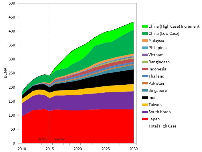
In an increasingly LNG-connected world, Russia’s strategic position is impacted by global gas market fundamentals. This is despite (or perhaps because of) Russia’s pre-eminent position in terms of gas reserves, export markets and productive potential. Chart 1 shows the global LNG balance from 2008 to 2030 in schematic fashion. The dashed line represents global LNG supply from existing and FID’d projects. The period to 2020 sees a huge increase in supply from the US, Australia and other projects. Asian demand in this timeframe is uncertain (Chinese economy and Japanese nuclear restarts in the main); the space between the Asian demand bar and the dotted line represents LNG which will flow to Europe.

Chart 1: Global LNG Balance

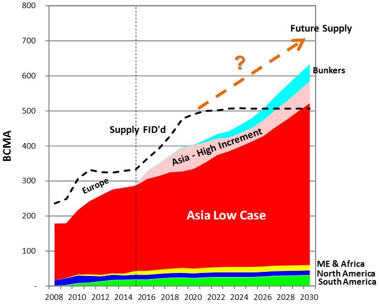
Source: Howard Rogers, OIES

In the recent past Russia has dismissed the US shale gas boom as a short term, unsustainable phenomenon. Russia strategic focus has been pre-occupied with the long-running Ukraine transit imbroglio, frequent adaptations of its plans for South and North Stream pipelines and its response to the DG Competition inquiry. But Chart 1 suggests that the threat of a surge of European LNG imports has probably now become a ‘real and present danger’ to Gazprom’s European gas market share. On a cost basis, Gazprom’s supplies to Europe are very competitive as shown in Chart 2.

Chart 2: Comparison of Russian Pipeline Gas, US and Non-US LNG delivered to Europe

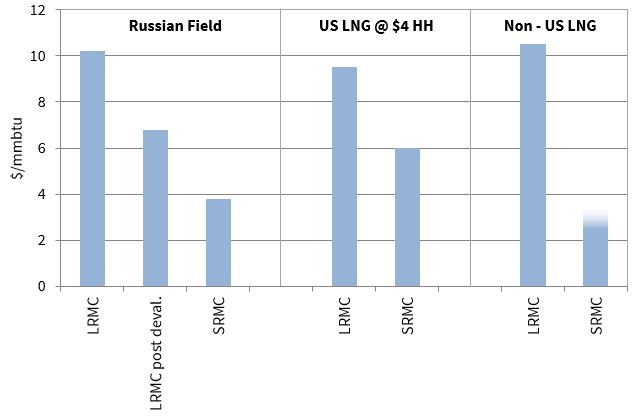
Source: J Henderson & D Ledesma, OIES

Chart 2 shows the long run marginal costs of ‘new’ West Siberian Gas in the range of $10/mmbtu (pre rouble devaluation) to $6.50/mmbtu (post rouble devaluation). But this is academic as it already has some 100 bcma developed which could flow to Europe border and cover variable costs and export tax at a border price of $3.80/mmbtu.

Once competing LNG projects are FID’d and committed however, they will flow at short run marginal costs of ‘Henry hub plus shipping and regas costs’ in the case of US projects and probably just shipping and regas costs in the case on non-US projects. Russian adherence to oil-indexed pricing to date has arguably encouraged competing LNG projects. Will it now adapt its price-volume strategy to limit further competition from new LNG?

How may Russia respond to lower prices and competing supply?

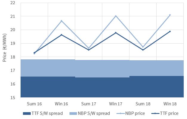
Gazprom has to date required its European mid-stream buyers to take delivery of (at least take or pay) contractual volumes at prices linked to oil-products. The majority of these contract volumes are delivered at border flange delivery points. Gazprom has however negotiated ad-hoc concessions and rebates relative to hub prices, to ease cost pressure on suppliers. This model is illustrated in the upper section of Chart 3.

Chart 3: Alternative Russian Contractual Sales Strategies

Source: Howard Rogers

Gazprom’s in-house marketing and trading capability gives it the option to pursue an alternative strategy in response to the emerging gas supply glut. The first logical steps would be:

Move delivery points to the existing European gas trading hubs
Move contract pricing terms to hub pricing
Meet buyers’ nominations with a mixture of physical gas transported from West Siberia and gas bought off the hubs.

This is termed the ‘hub re-delivery model’ and is already used in UK medium terms contracts. It is depicted in the lower half of Chart 3.

In this manner Russia could influence the level of European hub prices through taking control of the scale of physical gas transported to the European gas market. Keeping European hubs (and by arbitrage Asian LNG spot prices) at prices below those supporting new LNG projects, acts to deter competing supply.

Over time the currently anticipated LNG ‘glut’ will be absorbed by a combination of Asian and new market LNG demand. Europe also faces the need to offset domestic production decline in Europe with new imports. As a result it is reasonable to expect European hub prices to rise again as these factors take effect into next decade. Gazprom then has another important strategic choice:

If Gazprom allows European hubs to exceed $9 to $10/mmbtu, new LNG projects will achieve FID. Once new projects are launched, production SRMC is then very low.
If Gazprom increases exports to keep European hubs below $9 to $10/mmbtu, new LNG FID’s will likely be delayed.

These dynamics leave Russia in a very strong position to dominate the sale of incremental gas supplies into Europe.

Pulling back to the bigger picture, it is worth noting that any idea on Russia’s part of compensating for disappointing European sales/prices by threatening to take its gas to Asia is flawed:

Eastern Siberian gas is ‘stranded’, it is not connected by infrastructure to European markets,
West Siberian gas delivered by the Altai line to China would be 30 bcma of the 100 bcma of ‘surplus productive capacity’; this would not impact deliveries to Europe,
Additional supplies of Russian gas to Asian markets, whether pipeline gas or LNG, all other things being equal, merely displaces an equivalent volume of LNG from those markets which would likely end up in Europe.

As yet it is unclear whether Russia recognises the challenges set out above and is willing to adapt its strategy accordingly. But look out for changes in long term pricing terms and delivery points to hubs as the first signs of such a move.

Article written by Howard Rogers, David Stokes & Olly Spinks

Global LNG and European gas workshop

Timera Energy offers tailored workshops exploring the evolution of the global LNG and European gas market fundamentals and pricing dynamics. These workshops involve Howard Rogers who, as the Director of the Gas Programme at the Oxford Institute for Energy Studies, is acknowledged as a leading industry expert in the global gas market.

If you are interested in more details please email olly.spinks@timera-dev.positive-dedicated.net

Implied vs historical gas price volatility

Posted on November 16, 2015January 16, 2020 by David Duncan

European gas hub markets are maturing. This can be seen via the increase in range and liquidity of traded products. Growth in trading activity is focused on the UK NBP and Dutch TTF hubs, with TTF challenging the traditional dominance of NBP.

Consistent with maturing hub markets is a growing liquidity in traded gas options. There has also been growth in the penetration of shorter term flexible capacity products which contain embedded optionality (e.g. gas storage capacity). This means that gas price volatility is becoming a more transparent driver of value in energy portfolios.

In today’s article we look at two different volatility benchmarks (historical and implied). We also do a practical comparison of the evolution of these benchmarks over the last three years and consider their impact going forward.

Historical vs implied volatility – the basics

If you are familiar with these measures of volatility feel free to jump ahead to the next section.

Historical volatility

Historical volatility involves a retrospective calculation based on observed market prices over a defined period in history. It is a statistical measurement of the realised price dispersions of a specified contract over a specified time period. For example: “Day-Ahead volatility in Apr 2015 was 55%”.

Historical volatility is measured based on a dataset of realised historical price return observations. The wider the distribution of historical price returns, the higher the volatility measurement (and vice versa).

Implied volatility

The level of volatility expected by the market can be ‘implied’ from the prices of traded gas options. For example: “the Jan 2014 ICE NBP gas call option contract has an implied volatility of 50%”.

The key to being able to imply volatility from traded asset prices is that the level of volatility is an input into the standard pricing formula (e.g. Black Scholes) used to value optionality. Option prices are a function of strike price, underlying gas price, time to expiry and volatility. So if the price of an option is known, then implied volatility can be backed out using the option pricing formula.

Applications of historical vs implied volatility

The key advantages of historical volatility as a measure are its transparency and objectivity. There are minor variations in the way that historical volatility is calculated, but it represents a relatively simple and accessible statistical measure.

EnergyStock, the Dutch fast cycle storage operator, has recently started publishing a volatility dashboard which contains a set of historical volatility indices on TTF gas prices. The dashboard provides a new and useful source of data on rolling and annual indices for the TTF day-ahead and month-ahead contracts.

Publication of reliable volatility indices is an important step in developing market liquidity in products with embedded optionality. Gas traders need middle office sign off in order to do any transactions. And middle office in turn require an independent & objective volatility benchmark for P&L and risk measurement calculations (either as a simple input to benchmark the value / risk of vanilla option portfolios or as guidance for stochastic parameters required for more complex flex valuation models). Most speculative trading companies (e.g. hedge funds) do not permit traders to take exposures in a market until there is an established objective risk benchmark.

Robust implied volatility benchmarks have only recently emerged in the European gas market. The reason is that the meaningful measurement of implied volatility requires a critical mass of traded option liquidity. Implied volatility indices are well established in the oil market (e.g. the CBOE OVX index). But it is only over the last 3 to 4 years that gas options liquidity in Europe has supported the measurement of implied volatility.

The advantage of implied volatility over historical volatility is that is represents a current (forward looking) market view on the level of volatility. As such, reliable implied volatility data is highly valued by traders and risk managers.

Gas options price data is harder to come by than straight gas price data (used to calculate historical volatility). Marex Spectron, Europe’s leading gas options broker, has been developing a comprehensive dataset* covering volatility surfaces for key NWE hubs. ICE also publishes an implied volatility surface for the NBP and TTF hubs but the Spectron surfaces more accurately reflect the current market. This is because they include option bid / offer data where as the ICE implied volatilities are only based on the traded option prices on the exchange (some of which can be quite stale given sparse liquidity across some strike / maturity combinations). We have used this dataset in the next section to run a numerical comparison of historical vs implied volatility.

Running the numbers on NBP volatility

Chart 1 shows a comparison of:

Historic 30 day rolling volatility on the ICE NBP Month-Ahead Futures contract
Implied volatility from ‘at the money’ Month-Ahead NBP gas options

Chart 1: NBP month ahead volatility benchmarks

This comparison provides an interesting illustration of the different characteristics of historical vs implied volatility. The most obvious initial observation is that implied volatility is generally higher than historical. This is because implied volatility incorporates a risk premium (reflected in the option price) as well as capturing within day price movements (historical volatility is calculated off a single end of day price).

Chart 1 also provides some interesting examples of how the two measures of volatility react to market events. Take the March 2013 NBP gas price spike as an example. The reaction of implied volatility to market events is immediate. The prices of options rise as risk premiums increase as can be seen with the spike in implied volatility in Mar 2013 on the chart. The impact of a market shock on historical volatility is more delayed as it feeds through the historical gas price series used to calculate volatility.

A jump in implied volatility can disappear as quickly as it came. This can also be seen in Mar 2013 where implied volatility rapidly returned to previous levels as new supply was diverted ensuring the market impact was temporary. The historical volatility series however averages in the impact of the price spike as long as higher gas prices remain in the historical 30 day price data window.

These characteristics do not necessarily mean implied volatility is a more reliable measure. Implied volatility represents an expectation of average volatility up until expiry, so can fluctuate significantly closer to contract expiry. Implied volatility is also dependent on the consistent availability of reliable options price data. Limited data over a given period can produce spurious changes in volatility.

Implied volatility benchmarks can be of limited use as a source of direct input data for complex pricing models. These models can require a number of non intuitive parameters far beyond simple implied volatility benchmarks (limited to standard option products). For example, a gas storage model may use spot volatility, mean reversion and price jump diffusion parameters to describe stochastic price behaviour. There is no clean method to generate these parameters from a single monthly implied volatility benchmark.

Volatility set to become increasingly important

As the European gas market continues to evolve, understanding the impact of volatility on asset value will become increasingly important. European energy portfolios have large underlying exposures to the level of gas price volatility. For example flexible volume customer contracts, pipeline swing contracts, storage capacity and transport capacity all contain embedded optionality, the value of which is driven by volatility.

The evolution of the benchmarks we have referred to is providing increased market transparency on the level of gas price volatility. Take a look at other more mature commodities markets (e.g. oil & metals) for an indication of the way forward. Gas hub prices are already firmly ‘on the radar’ of most industry participants. Gas price volatility levels are soon to follow.

Article written by David Stokes & Olly Spinks

*For more information about the Spectron implied volatility data please contact Richard Frape.

Last week’s UK power price spike

Posted on November 9, 2015January 16, 2020 by David Duncan

The tightening UK system capacity margin has been a theme of this blog over the last 4 years. This manifested itself last Wednesday in a period of magnified system stress and spiking power prices. The system operator, National Grid, took a number of defensive actions, paying up to 2500 £/MWh in the balancing mechanism to bring capacity online and ensure continuity of supply.

The issues last Wednesday related to a specific set of circumstances, but these were by no means an extreme event. High demand was not the issue. Several thermal asset outages combined with reduced interconnector flows and very low wind levels to cause the capacity squeeze.

System stress eased as capacity came back online with little impact on forward prices. But Wednesday’s events are an indication of more to follow as the system capacity margin continues to tighten over the next two winters.

The more enduring impact of this event is likely to come from the news headlines it attracted. It is this unwelcome media attention that is set to increase the UK government’s focus on security of supply, particularly as more plant closures loom in 2016.

The spike deconstructed

Chart 1 illustrates UK generation output on Wednesday in the context of the three proceeding days. Demand conditions were relatively benign, with peak demand lower than Monday or Tuesday. Wind levels were low across last week, but particularly low on Wednesday (with output falling to less than 1% of potential). The impact of coal unit outages and a reduction in French interconnector flows can also be seen.

The combination of these events was unusual but not extreme. But the market price impact was magnified by the UK’s low system capacity margin.

Chart 1: UK generation output Wednesday 4^th Nov

Source: Timera Energy (data from Gridwatch)

National Grid issued a Notification of Inadequate System Margin (NISM) at 13.30, a fairly rare event (the last being in 2012). The NISM called for an additional 500 MW of capacity across the 16:30-18:30 period. Grid then took a number of balancing and reserve actions to address the shortfall, including procuring capacity at up to 2500 £/MWh in the balancing mechanism. It also resorted to the ‘last resort’ use of 40 MW Demand Side Balancing Reserve contracts across the 18:00-18:30 period (a mechanism we explain in more detail below).

The prices last Wednesday can be seen in the context of adjacent days in Chart 2. The red and blue lines show the balancing mechanism system sell and system buy prices respectively. There are indications of some system stress via balancing prices on the two preceding days (given low wind levels and thermal outages). But the balancing price shock became much more pronounced on Wednesday as Grid took more aggressive actions to procure capacity.

Chart 2: UK prompt power prices around Wed 4^th November

Source: Timera Energy (data from Elexon and N2EX)

This in turn fed through into higher day-ahead power prices (in the N2EX auction) on Wednesday, shown by the black line. However the temporary nature of this event can be seen as conditions reverted back to more normal levels on Thursday.

Chart 2 also shows the UK balancing mechanism transitioning from a dual to a single cashout price from 5th November. This one of a number of measures being implemented over the next couple of years under the supervision of Ofgem to ensure sharper balancing price signals in the UK power market.

The events of last week are empirical evidence of a tightening system capacity margin causing higher and more volatile prompt prices. This is exactly the sort of situation that we foreshadowed in the final sentence of our article UK capacity new build challenges two weeks ago.

Reserve capacity buffer is increasingly important in the UK power market

Price spikes do not necessarily reflect the imminent threat of blackouts, despite last week’s news headlines suggesting otherwise. This is because Grid (under the supervision of the UK government) has implemented a mechanism to procure a buffer of emergency reserve capacity. This emergency reserve buffer comes in two categories:

Supplemental Balancing Reserve (SBR) – provided by older power plants that agree to be withdrawn from the wholesale energy market in exchange for payments as reserve capacity
Demand Side Balancing Reserve (DSBR) – provided by large energy users who are able to reduce their demand during peak periods in exchange for payments

Grid has contracted 2.5 GW of reserve capacity under these mechanisms for the coming winter (2015/16). This volume is dominated by SBR (less than 200 MW of it is DSBR), which is provided by aging power plants. A total of 8 plants have been contracted to provide SBR, all of them on the ‘endangered species’ and hunting for any form of return to contribute to fixed cost recovery.

This buffer of SBR/DSBR reserve capacity has become the key tool to manage the UK capacity crunch. From a security of supply perspective SBR acts to reduce the risk of blackouts. It is therefore included in Grid’s calculations of system reserve margin, which is almost zero without it.

But because SBR can only be called as a last resort, it does not prevent sharp rises in prompt power and balancing prices during periods of system stress. Events such as last Wednesday are evidence of this in action, but only a prequel to a much tighter market as capacity continues to close in 2016.

The UK capacity market is yet to deliver a price signal that covers the fixed costs of existing CCGT capacity (let alone the delivery of new capacity). That shifts the focus of plant owners & investors on to the energy and balancing markets. But investment decisions are not made based on volatile balancing prices alone.

A recovery in forward market generation margins (sparkspreads) is required to stem the tide of plant closures and encourage new investment. And as the system capacity margin continues to tighten, it is only a matter of time until the UK forward curve starts to reflect higher returns in the prompt market.

Article written by David Stokes & Olly Spinks

UK capacity price may clear in single digits

Posted on November 2, 2015January 16, 2020 by David Duncan

The system reserve margin in the UK power market is at an unprecedented level of tightness coming into the second capacity market auction in December. Last year’s inaugural capacity auction delivered little in the way of new capacity. In fact the low auction clearing price (19.40 £/kW) crystallised the economics of a number of older thermal plants which have since indicated they will close. So whatever the outcome of the 2^nd capacity auction next month, the system reserve margin is set to tighten further into winter 2016.

If you had no knowledge of the UK power market and somebody explained this landscape to you, what would you anticipate would be happening in the capacity market? You would probably assume that prices would clear at a level that prevented the further closure of existing plants. You may even expect a capacity price that incentivised the delivery of large scale new capacity build. Our take on the second capacity auction is that neither of these things are going to happen.

The 2^nd auction is for delivery of capacity over the Q4 2019 to Q3 2020 period. As for any market, the auction outcome is driven by the interaction of supply and demand. Demand is determined by the government’s capacity target. Supply is driven by a prequalification process where different sources of capacity are accepted into the auction subject to a defined set of conditions. A firm view on the volume and type of prequalified capacity only became available two weeks ago. So with this in hand we now have all the information required to undertake a robust analysis of the 2^nd auction outcome.

In this article we provide an overview of:

The auction supply and demand balance
New factors in play this year
The drivers of capacity price outcome
Our view on capacity price range in the 2^nd auction
The broader implications of the auction outcome for the UK power market

As for last year, the information in this article is a higher level summary of more detailed analysis that we have undertaken of auction drivers and pricing dynamics. Detailed projections of the 2^nd auction pricing dynamics and implications for the UK power market are available in our client briefing (details below).

Supply & Demand balance

The 19.40 £/kW capacity price in the 1st auction last year was well below the market consensus view (around 45 £/kW). This outcome was driven by an oversupply of existing capacity relative to the government’s demand target. These conditions remain in the second auction.

The government’s demand target is 44.6 GW this year, with a similar demand curve structure to last year where demand varies depending on clearing price. Demand increases by up to 1.5 GW above the target at zero price, or decreases by up to 1.5 GW below the target at the 75 £/kW price cap. The demand curve can be seen in Chart 2 below.

On the supply side, there is around 50GW of existing capacity (including capacity that is already committed and under construction). So the market is oversupplied again this year and this will again act to supress prices, in the absence of a material shift in the bidding behaviour of existing plant owners. An overview of the supply and demand balance is shown in Chart 1 which breaks down supply by capacity type.

Chart 1: 2^nd capacity auction supply & demand summary view

Source: Timera Energy

What’s new in this year’s auction?

If you are not particularly interested in the drivers of capacity pricing and just want a view on market outcome then you can skip to the next section.

In this section we focus on five important factors that change the competitive landscape in the 2^nd auction. There are also a number of more technical rule changes that have been implemented into the second auction. These are not dealt with in this article.

Interconnectors: This year’s auction has an additional 2.4 GW of de-rated interconnector capacity that was not eligible to participate last year. Interconnectors have been included in the auction on the basis of quite steep capacity derating factors to reflect flow uncertainty. But both existing and new interconnectors will likely be bid at zero price, given healthy energy margins (driven by higher UK power prices vs those on the Continent) and other regulatory support (e.g. the cap & floor revenue structure). In other words inclusion of interconnectors will act to displace existing capacity.
Supply reduction: 7.6 GW of existing capacity has opted out of the 2^nd auction. 5.8 GW of this capacity has opted out because owners have indicated an intention to close plants by the delivery year (2019/20). In addition there is 3 GW of capacity from last year’s auction that will not participate this year given it received 3 year refurbishing agreements (EDFs Cottam and West Burton coal units). The removal of these plants from the auction has significantly reduced the number of older thermal plants from the capacity supply stack. This makes analysis of this year’s auction somewhat easier.
New build penalties: Only one new CCGT was successful in last year’s auction. We have written about the problems encountered by Carlton Power’s Trafford CCGT project. As a result of the issues with the Trafford project, the government has introduced a range of stronger penalties for owners which fail to meet their capacity obligations. In practice this means that new build CCGT projects are likely to bid at higher price levels than in last year’s auction. In fact in an oversupplied market, we would be very surprised to see any new build CCGT project successful in the 2^nd auction, aside from the 810 MW Carrington CCGT project which is already under construction and is therefore capacity price insensitive.
Bidding behaviour: The other important factor that influences this year’s auction is clearer information on competitive bidding behaviour. There is a bidding track record from last year that is useful in inferring how owners may bid assets this year. This is particularly important for the older coal and CCGT assets that are likely to dominate marginal price setting in the auction. We know which generation units bid above and below last year’s 19.40 £/kW clearing price. We also know that:
1. Forward market energy margin conditions for CCGT plants are broadly similar to those going into last year’s auction (suggesting that CCGT bidding behaviour may be similar).
2. Forward energy margin conditions for coal plants have deteriorated as dark spreads have declined with falling power prices in 2015 (suggesting that coal plant owners may bid at relatively higher levels than last year).
Marginal bidding: The other dynamic demonstrated by last year’s auction outcome is that unless owners are prepared to close their plant if their bid is unsuccessful, they are strongly incentivised to bid zero. In other words capacity bids are likely to reflect the true incremental return required to keep assets open. This dynamic is important coming into the second auction because it appears to us that the volume of capacity that is likely to bid at (or close to) zero price comes close to meeting the government’s demand target.

The five factors above combine to play an important role in driving the dynamics of the second auction outcome.

Auction result comes down to older coal & CCGT plants again

We developed a comprehensive analytical tool kit for analysis of the UK capacity market in the lead up to the first auction last year. We used this to publish a client report in mid-November 2014 that contained the following key conclusions on the 1^st auction (quoted from the Executive Summary):

“Marginal plant: 3 key plant types are likely to drive the 1st auction outcome (older coal, older CCGT, low capex peakers).”

“Pricing: Our analysis indicates a 1st auction capacity price around 30 £/kW if participants bid rationally to recover costs. But the 1st auction outcome will come down to EM (& CM) expectations (diverse range likely across players).”

“Downside risk: The low 1st auction target and ‘Fear of Missing Out’ dynamics may lead to a lower clearing price than expected. These factors could easily combine to reduce the 1st auction clearing price by 5-10 £/kW.”

These dynamics remain relevant into the 2^nd auction but with greater pressure on prices. In order to provide an overview of 2^nd auction pricing dynamics we start with a supply and demand chart. It is important to note that Chart 2 does not represent our projection of the auction outcome (as was inferred by several readers when we published a similar chart last year). This is reserved for our client briefing. Instead it shows a credible scenario based on groupings of assets into categories.

Chart 2: A grouped plant 2^nd auction scenario with a 10 £/kW capacity price

Our modelling framework allows the analysis of pricing dynamics at an individual asset level. But for the purposes of this, we consider market dynamics based on the grouping of plants of similar technology, age and efficiency. This helps in demonstrating the key drivers of marginal pricing dynamics.

The first observation from Chart 2 is that there is a large volume of ‘price insensitive’ capacity bidding around zero price. This is made up of existing capacity that owners do not intend to close by 2019/20, regardless of capacity price outcome.

For example, it includes existing hydro, nuclear, interconnectors, peakers/DSR, higher efficiency coal and mid to high efficiency CCGTs. It also includes new interconnectors, the 810 MW Carrington CCGT (under construction) and around 500 MW of small scale new build peakers and DSR (assumed to be economic based on other revenue streams e.g. ancillaries & triad avoidance revenue). In the scenario shown, this capacity makes up around 43 GW of the 44.6 GW target. That does not leave much room for a high capacity price outcome.

It is likely to be the plants sitting directly to the right of this price insensitive tranche in the supply stack that determine the outcome of the 2^nd auction. Like last year these are likely to be a mix of lower efficiency coal and CCGT plants, interspersed with more competitive new peaker/DSR projects.

But if our assumption of around 43 GW of price insensitive capacity is correct, there may only be a requirement for two or three additional thermal plants to clear the auction. In volume terms a maximum additional capacity of 3 GW would be required to clear the auction, from an overhang of about 7 GW of existing capacity and maybe 1-2 GW of competitively priced new peaking/DSR capacity. It is this level of competition around the margin that is in our view set to supress prices.

Capacity price outcome & bounds

We think the capacity price is likely to fall within a 0-25 £/kW range. The upper bound of this range is driven by the fixed cost recovery of less efficient CCGTs. There are around 5 GW of these plants competing around the margin and it is our view that a significant portion of this capacity will be priced at or below fixed costs (given capital costs are already paid down). In other words if the auction price rises to the 25 £/kW level there is likely to be more than enough supply to clear the auction.

The lower bound is more complex. It could be that there is enough price independent existing and new capacity to clear the auction at zero. However we suspect that the owners of marginal older assets may baulk at bidding units so low. This is because:

The alternative option to bid capacity into the T-1 auction (in 2018) looks increasingly attractive as existing capacity continues to close in the absence of a new build price signal.
The big six utilities have a portfolio consideration where it may make sense to bid marginal assets at positive prices to increase the capacity price return across the rest of the portfolio (even if it means the marginal plant are unsuccessful in securing a capacity agreement).
By accepting a capacity agreement in the Dec auction at zero price, owners forfeit the option to close before 2020. That option has some value for marginal older plant and is likely to be reflected in positive bid prices.

So while the risks remain to the downside in this auction given the overhang of existing capacity, we would be surprised to see a zero price outcome.

Where could we be wrong with the logic set out above? The biggest risk is around the volume of price insensitive capacity we have assumed (e.g. 43 GW in the scenario in Chart 2). If that volume is higher e.g. due to a higher volume of competitive new build peakers/DSR, then it pushes price risk further towards the downside. If the volume is lower, then it reduces the overhang of capacity competing to clear the auction. But we struggle to see a margin of error that absorbs the 5 GW+ overhang of CCGTs and competitively priced new peakers/DSR capacity.

Broader implications for the UK power market

If there is another low capacity price outcome in the 2^nd auction we would expect a continuation of the fallout from the 1^st auction. This may mean the closure of another 2-4 GW of lower efficiency coal and CCGT units (on top of the plant closures already announced). That would leave the UK power market in a precarious state.

The chances of rolling blackouts have fallen with the implementation of the Supplementary Balancing Reserve (SBR) mechanism managed by the system operator (National Grid). Contracted SBR capacity acts as a buffer of emergency reserve and Grid will presumably step up the purchase of SBR capacity as the system reserve margin heads towards zero. What is unattractive about this outcome is that SBR risks becoming a proxy capacity market, but one that lacks a robust and transparent rule book.

However, SBR capacity (given its emergency status) should not stand in the way of higher and more volatile power prices as plants continue to close. This appears to be the path down which the government is steering the UK power market, whether intentionally or otherwise. And that would provide a rare glimpse of blue sky through the fog of EMR policy intervention. Sharper price signals in the wholesale energy market are exactly what is required to address the impending capacity shortage.

This article was written by David Stokes & Olly Spinks

2^nd Auction Client Briefing

We are offering a client briefing service that provides a more detailed analysis of the 2^nd auction dynamics, pricing outcome and implications for the wholesale power market and future capacity auctions. This service also includes a conference call to discuss analysis and any specific issues of relevance.

If you are interested in more details please email david.stokes@timera-dev.positive-dedicated.net

Global gas price evolution: 5 key drivers

Posted on October 26, 2015January 16, 2020 by David Duncan

The global gas market has been turned on its head over the last 18 months. In Q1 last year, Asian spot LNG prices were breaking records with the Platts JKM marker above 20 $/mmbtu. Behind this was a structural divergence across regional gas prices in Asia, Europe and the US, with flexible LNG supply diverted to Asia to cash in on premium prices. The market consensus view was that market tightness and higher gas prices were here to stay.

Fast forward to Q4 2015 and global gas prices have slumped. Asian and European prices have rapidly converged in a relatively tight range above 6 $/MMBtu. US gas prices remain below 3 $/mmbtu, but the price differential between the US and Europe is gradually being eroded by oversupply. The approaching northern winter, usually a driver of higher seasonal prices, has failed to have an impact so far.

We pointed to the start of a new phase of global gas market oversupply in September 2014. But what are the drivers that are going to determine the dynamics and duration of this new phase and the evolution of gas prices into next decade? We set out the five key factors that we are watching below.

1. Impact of crude pricing

Oil-indexation remains a powerful influence on European and Asian gas prices. In Asia, almost all LNG contract volumes are indexed to crude benchmarks (e.g. JCC, Brent). In Europe, despite a much publicised trend towards the spot indexation of gas, the majority of long term pipeline swing contracts also remain indexed to oil (primarily gas oil & fuel oil) – albeit moderated via price formula concessions and rebates which have become prevalent post 2008

Oil-indexation has a particularly important influence on spot prices in Asia and Europe because of its influence on the exercise of contract volume flexibility. The ability to vary swing contract take is optimised based on the differential between oil-indexed contract prices and spot gas prices. When spot gas is cheaper than oil-indexed contract prices, contract volume take is reduced (and vice versa).

This means that oil-indexed contract prices act as an important longer term anchor for gas prices. This relationship is a loose one over a shorter term horizon given the influence of other supply and demand factors. But oil-indexed prices act as a ‘magnetic ceiling’ and typically draw spot gas prices back in line in a reasonably balanced market. That said, a very tight market can see spot gas prices ‘break through’ this ceiling (UK in 2005/2006) although such occurrences are rare and transitory. Alternatively an oversupplied spot market can see hub prices disconnect below contract prices (e.g. as in 2009-10).

On this basis, the length and depth of the current decline in oil prices is a key factor that will determine how gas prices behave into next decade. We have recently set out our view on oil prices. Crude prices should recover over time given they are currently well below LRMC benchmarks. But there may first need to be a period of lower prices to interrupt the US shale oil investment cycle.

2. Asian LNG Demand

Asia represents the main source of uncertainty on the demand side of the global gas market. In summary across the large and growing Asian gas consumers:

Japan: Lack of clarity on the pace and scale of nuclear restarts
South Korea: Uncertainty around gas vs coal usage in the power sector
India: Questions over infrastructure, domestic pricing and affordability of gas vs coal

That leaves the most important market China. The key source of uncertainty around Chinese demand is the scale of potential demand growth. China’s LNG requirements are the ‘balance’ required after:

Domestic production (uncertain volumes of conventional, shale, coal bed methane and syngas from coal)
Pipeline Imports from Turkmenistan, Central Asia & Myanmar
Russian pipeline gas from Siberia

We know demand growth will be large. But the difference between large and very large has a substantial impact on the global gas demand. It is also unclear how Asian demand (particularly from buyers with lower contract cover like China and India) will respond to lower spot LNG prices. We illustrate the uncertainty around Chinese LNG demand via an illustrative ‘high’ and ‘low’ LNG demand growth case in Chart 1.

Chart 1: Asian LNG demand growth scenarios

Source: Howard Rogers OIES

3. European demand recovery

European gas demand has fallen almost 20% this decade. Around half of this decline occurred in 2014 due to an outlier warm weather year across Europe. Weather normalisation aside the main drivers of the evolution of European demand are the rate of economic growth and the extent to which there is a recovery in gas fired power plant load factors.

Two illustrative scenarios are shown for ‘steady’ vs ‘low’ gas demand growth in Chart 2.

Chart 2: Illustrative European gas demand evolution scenarios (includes Turkey)

Source: Howard Rogers OIES, Timera Energy

The ‘steady’ growth scenario assumes:

Some SRMC driven coal gas switching as gas hub prices fall (particularly in UK)
Emissions legislation driven retirement of coal plant (LPCD & IED)
Planned retirement of nuclear plants (Germany important)
A slowdown in renewable investment over the next decade

The ‘low’ case assumes:

Coal remains ahead of gas in merit order
Some coal & nuclear retirements delayed
Renewables investment pace maintained
No effective carbon pricing mechanism

The more than 100 bcma difference in demand by 2030 illustrates the uncertainty involved.

4. Impact of new liquefaction capacity

There is more than 150 bcma of liquefaction capacity that has already reached Final Investment Decision (FID) sign off and is set to be built by the end of the decade. 140 bcma of projects are already under construction, with more than 55 bcma due to be commissioned by the end of 2016, across Australia, Malaysia, Indonesia and the first US export trains at Sabine Pass.

We have written in some detail about the mountain of new LNG liquefaction capacity that is being developed. So we won’t labour the point in this article. But suffice to say that current oversupply in the global gas market is in large part due to the overhang of committed new capacity.

5. Russian response to oversupply

There is no OPEC in the gas market. But Russia is certainly large enough to influence the global market balance. Particularly important will be how Russian producers (primarily Gazprom) react to the growing global oversupply of gas.

The challenge Russia faces can be broken down into two key Issues:

Russia’s price / volume strategy in Europe
Russia’s influence on timing of new LNG project investment decisions

As global LNG supply increases, European LNG imports are set to rise as Europe’s hubs absorb gas as a market of last resort. These import volumes have the potential to push global gas prices down towards US Henry Hub levels. But Russia has the ability to support hub prices via influencing the volume of gas it sells into Europe. It can achieve this via granting a range of (likely temporary) concessions on its contract prices (as seen in 2011-13). This Russian price/volume strategy may be a key factor determining how deep and prolonged the current price slump will be.

Looking into next decade, as the surge in Australian & US LNG exports is absorbed, the global gas market will tighten again and hub prices in Europe will rise. This leaves Russia with an important longer term strategic challenge:

If Gazprom allows hubs to exceed $9 to $10/mmbtu, new LNG projects will achieve FID. Once launched the SRMC on these projects is very low.
If Gazprom increases exports to keep European hubs below $9 to $10/mmbtu, new LNG FID’s will be delayed. This would appear to be sensible strategic behaviour but may be hard to sustain, particularly in a world of significant oil price recovery.

Making sense of the global gas market

In our view there is little merit in trying to analyse the global gas market on a ‘bottom up’ basis (i.e. by trying to build up a robust view of all individual sources of supply and demand). Changes in the 5 key factors set out above mean that analysis at this level of detail is spurious at best.

Instead we take a ‘top down’ scenario based approach where we group key tranches of global supply and demand. We focus particularly on:

the key tranches of flexible supply that drive marginal pricing
the interaction between prices across different regions to clear the global market
potential ranges in the evolution of demand by region
the overlay of strategic considerations from large market players with pricing power (e.g. Russia and China)

The attraction of this approach is it is easily digestible and transparent. But our analysis points to the fact that the influence of Russian strategic decisions are more important than is often recognised. So in an article to follow shortly, we will return and explore Russian price/volume strategy in more detail.

Global LNG and European gas workshop

If you are interested in more details please email olly.spinks@timera-dev.positive-dedicated.net

Article written by David Stokes, Howard Rogers & Olly Spinks

The UK CCGT new build challenge

Posted on October 19, 2015January 16, 2020 by David Duncan

Carlton Power was the only bidder in the UK’s first power market capacity auction that secured a capacity agreement to build a new CCGT (in Dec 2014). Carlton Power’s Trafford CCGT, a 1520 MW project in Manchester, received a 15 year agreement at the clearing price of 19.40 £/kW.

But the Trafford plant was bid into the capacity auction without finance and without a long term tolling agreement to back it. An interview Carlton Power did with the Telegraph last week suggests that the project is struggling to secure an offtake contract and financing and may not be able to deliver against its 2018/19 capacity agreement.

The problems associated with Trafford highlight the challenges that CCGT developers face given current weakness in generation margins. A 19.40 £/kW annual capacity payment barely covers the direct fixed costs of a new CCGT. So making a Financial Investment Decision on a new plant means finding someone to take on the market risk around the substantial recovery in energy margin required to make the project profitable. It appears that lenders and tolling counterparties are reticent to take on that risk.

Challenging economics at £19 capacity price

It has not all been bad news for CCGT project developers. They have benefited from falling capex costs as turbine manufacturers slash unit costs and bulk up guarantees in order to try and recover sales. Whereas 5 years ago benchmark CCGT costs were around 700 £/kW, project developers are now claiming costs can be reduced to around 500 £/kW.

But even with capex this low, our analysis indicates a generic new build CCGT project needs more than 40 £/kW under a 15 year capacity agreement in order to be economic. Chart 1 provides an overview of this analysis. There may be some benefits that specific projects can claim to reduce this (e.g. locational reduction of TNUoS), but these are unlikely to mean more than a 5-10 £/kW reduction in required capacity payment.

Chart 1: Illustrative UK new CCGT build economics at 500 £/kW

Source: Timera Energy

Tough to get a toll & finance

The big six UK utilities are the natural buyers of tolling agreements. But most of these portfolios already have significant existing exposure to CCGT margins via their own generation fleet. A number of utilities are also sitting on their own CCGT development options.

Historically, banks and commodity traders have also been potential tolling counterparties. But these players are pulling back on long term power price exposure driven by balance sheet constraints and tougher regulatory measures. This is contributing to the shrinking availability of market participants even willing to discuss longer term tolling contracts.

Market players are also increasingly wary of taking on tolling contract exposure beyond a 5 year duration. This is due to a combination of:

regulatory uncertainty (e.g. lack of clarity around SBR contracting, Capacity Market changes, abolition of LECs)
the threat of other new entrant capacity (e.g. peakers, interconnectors)
CCGT load factor erosion by renewables

That makes the financing of CCGT projects difficult. Lenders are looking for the security of a significant portion of net margin to be contracted over a 10-15 year horizon.

Capacity market issues

The Trafford experience has demonstrated a design issue with the UK Capacity Market. Developers can treat capacity agreements as an option to develop projects, contingent on securing finance & a toll. In the case of Trafford the cost of this option is around £8m which is quite small in the context of the scale of the project. The government has been quick to point out that there will be a range of new rules to discourage this in future.

If the Trafford project does not proceed, the UK market faces a 1.5GW capacity hole in 2018/19 that needs to be plugged via the year ahead (T-1) auction in 2017. The supply stack in this auction is likely to be considerably steeper given the limited number of options to deliver capacity at a year’s notice. It is also likely to favour peaker and DSR capacity providers.

But a more important issue is the closure of 5-10GW of coal and CCGT plants over the next 18 months as we have set out previously. Yet the Capacity Market is not sending a price signal that supports development of large scale new capacity this decade. This highlights the dependence of the Capacity Market outcome on government (& system operator) forecasting of the supply and demand balance in 4 years time. If they are wrong, then the second line of defence is the SBR mechanism (lacking transparency) and year ahead auction (limited supply).

The System Operator (National Grid) seems comfortable about the coming winter in their Winter Outlook published last week, despite noting a historically low system capacity margin of 5.1%. But that comfort comes from their ability to contract emergency reserve via the ill-favoured SBR mechanism.

We will come back to overview the outcome of this year’s capacity auction shortly. But like last year the capacity prequalification data shows the capacity market has more existing capacity than required by the government’s target level. So capacity prices are unlikely to provide much joy for new CCGT projects in December. Ultimately a lack of price signal from the Capacity Market is likely to play out in the form of sharper price signals in the wholesale energy and balancing markets.

Article written by David Stokes & Olly Spinks

Defending energy portfolios against a credit event

Posted on October 12, 2015January 16, 2020 by David Duncan

Last week we looked at the threat of a systemic credit event in energy markets. Market prices are flashing a warning signal about the capitalisation and interrelated exposures of a number of large commodity trading firms.

However you assess the imminence and magnitude of the current threat, historical evidence shows a clear track record of systemic credit events. We looked at the 2001-03 Enron collapse last week as a case study. The events at the peak of the financial crisis in 2008-09 are another example. So rather than waiting to see if ‘commodity traders 2015-16’ is the next occurrence, what defensive preparations can be made in advance?

Issues with credit risk management in energy companies are often rooted in the basics. For example:

Ensuring the robust definition & measurement of credit exposures
Making sure these are reflected in commercial decision making and the ongoing management of counterparty exposures.

Credit risk management problems are often driven by an under-resourcing of credit risk functions, given the perception that they are just a cost centre or administrative control function. There can also be challenges within large energy companies when it comes to managing credit risk within business units (e.g. trading functions) versus the management of broader corporate credit exposures.

On a day to day basis credit risk may appear relatively dormant compared to market risk. But every once in a while it rears its ugly head and the scale of losses can dwarf those of more closely regulated market risk exposures. This means that credit risk is all about robust and efficient practices that provide a structural defence. Ramping up a focus on credit risk once a credit event is already in motion smacks of closing the stable door after the horse has bolted.

Defence in two steps

Building a basic defence against credit risk can be broken down into two key parts: (i) measures in place at the time of transaction and (ii) measures taken on an ongoing basis during the life of the contract.

Time of transaction: Company credit policies should dictate which companies are permitted counterparties, and (via a system of exposure limits) to what extent. Within this policy framework, the application of a Credit Value Adjustment (CVA) ensures that credit risk is priced into transactions on a deal by deal basis. CVA is calculated on the simple principle that a buyer of poor credit standing gets charged more than a strong buyer.

The CVA attempts to quantify the appropriate credit risk premium (or discount, when buying – recognising that credit risk is symmetrical in forward exposures). Its use is twofold:

As a direct input into contract pricing
As the basis for an internal transfer (actual, into a credit reserve; or notional for management accounts) to provide ‘self-insurance’ against the statistically expected losses arising from the portfolio.

Additionally, an extension of the CVA calculation generates an ‘at-risk’ number (sometimes called ‘CVaR’). CVaR is used in assessing how much of a credit limit is utilised by a transaction, and how much risk capital is represented by the deal. CVA is becoming common practice in energy companies, helped by an increased regulatory focus (e.g. IFRS 13).

Ongoing management: On a continual basis through the life of the contract, various practical steps are taken to update the calculation of, minimise, and manage the ongoing exposure. This exposure may actually be getting worse with time, as market conditions and/or general corporate weakness affect the counterparty adversely and call their commercial performance into question.

These steps include clearing, netting, bilateral margining and calling for collateral. Importantly they typically depend on the contract being written with good credit support terms.

Ongoing management of credit risk also falls back on robust definition, measurement & reporting of credit exposures. This requires an effective capability to analyse the future evolution of credit exposure, for example incorporating techniques such as:

Potential Future Exposure (PFE): quantification of maximum expected credit exposure of a contract/portfolio for a given time horizon & confidence interval.
Credit VaR (CVaR): quantification of default loss for a given time horizon & confidence interval.

These techniques are the building blocks of tracking and managing credit risk on both an individual contract and a net portfolio basis. The stochastic measurement of PFE for an example hedging contract is illustrated in Chart 1.

Chart 1: PFE measurement example

Source: Amsterdam Complexity

Direct hedging: In addition to these steps Credit Default Swaps (CDS) also provide the ability to directly hedge exposures to larger counterparties. But these are less commonly used by energy companies to manage day to day contractual credit risk. This is in part due to the complexities associated with exposure matching, pricing and management of CDS in relation to the underlying credit exposure.

Backing up principles with practicalities

The defensive steps described above make for a good routine credit risk management discipline. But energy companies face a number of practical problems in implementing these. For example:

Default data: The analytical techniques outlined above (e.g. CVA, CVaR) require default data and other inputs that typically come from rating agency assessments. The 2008-09 crisis is riddled with examples of how rating agency analysis was found wanting (e.g. their analyses of capital adequacy). We would be surprised if similar issues did not arise during the next major credit event.
Default measurement: Even good-quality default data understate credit/performance risk in a commercial sector like energy because they relate to bond default, and companies fail to perform under ordinary commercial contracts before (if ever) they default on bonds.
Structural change: Many energy contracts have very long tenor, more so than in other industries. Looking back at events over the last decade (e.g. commodity supercycle, shale gas, financial crisis, Fukushima) illustrates that even ten years is a very long time. Structural changes in the industry over several years can systematically undermine the creditworthiness of large players or even whole sectors at a time.
One shot defence: Although the credit support tools exist for inclusion in contracts, it is surprising how often companies fail to bolster their long-term contracts fully or allow credit terms to be negotiated away. There is generally only one opportunity to do this justice.
Heritage: Some energy companies come to traded-market credit risk management from a retail/utility heritage. This can result in relative weakness and under-resourcing of credit risk management versus e.g. market risk management.

Common sense over black boxes

Analytical techniques such as CVA, CVaR & PFE can materially improve an energy company’s defence against major credit events. But relying too heavily on these tools can be dangerous as was illustrated in 2008-09.

Probabilistic methods to measure and price credit risk need to be applied in a transparent manner rather than as ‘black box’ number generators. Outputs also need to be challenged with a healthy degree of scepticism. If results cannot be demonstrated to company management via simple benchmarks & sense checks then it is likely that the methodology is the problem rather than the audience.

This leads to a final key element of credit risk management: stress testing. Systematic and carefully designed stress-test scenarios are vital in a regular, periodic programme of stress tests. Stress testing is a specific discipline with best practices of its own, but it is particularly relevant in credit risk management. A few obvious examples:

What is the impact of the default of your largest counterparty (or top 3; or a sector of counterparties with interconnected exposures e.g. commodity traders)?
What is the impact of counterparty default on key contracts, either from an individual asset or portfolio perspective?
If 1. and 2. seem mundane then ‘reverse engineer’ a scenario that causes major portfolio stress.
If unable to raise a sweat with 3. it is probably time to use a bit more imagination.

The creditworthiness of large commodity traders is likely to ebb and flow with the fortunes of commodity prices and broader credit market stress. But there is enough smoke on the horizon to justify a prudent review of credit risk management. In our view building a robust defence is about effective policy, CVA analysis & implementation and contract credit support at the time of transaction. Then on an ongoing basis this needs to be backed up by the measurement and management of credit exposures, bolstered with appropriate stress tests.

Authors: Nick Perry, David Stokes, Emilio Viudez Ruido

Watch out for a major credit event

Posted on October 5, 2015January 16, 2020 by David Duncan

It is often said that when the tide goes out on commodity prices we find out who’s been swimming without shorts on. The market smells trouble brewing amongst some large commodity trading companies. The most prominent of these, Glencore, has attracted plenty of attention over the last week. Since the latest commodity rout began in August, Glencore’s share price has slumped and the cost of insuring default risk has soared.

The focus on Glencore is partly because of its size, but also because it is one of the few publicly listed commodity traders. This means that there are much clearer market price signals for balance sheet stress. But Glencore’s exposure to falling commodity prices is far from unique. In fact the majority of global commodity traders have a similar business model. That means that trouble for one is likely to signal trouble across the sector. These companies are big energy market players and that brings credit risk sharply into focus.

For the energy industry, the echoes of Enron’s collapse in 2001 are sufficiently loud that they are worth revisiting. In this article we look at the credit risk issues that are rapidly evolving in the current market. But we do so in the context of looking back at the Enron driven credit event as a case study for what may happen next. We will then return next week and consider what’s to be done about it from a credit risk management perspective.

What’s all the worry?

Glencore and its commodity trading peers, companies such as Vitol, Trafigura, Noble & Mercuria, have evolved their business models substantially over the last 10-15 years. Growth has been fuelled by a big bull market in commodities. As an example, Vitol (the world’s largest oil trader) had zero profit in the late 90s but ballooned to a $2.28bn profit by 2009.

Commodity traders have expanded their core trading business by backing it with large asset portfolios in an attempt to claim margin across the supply chain. This has meant business model evolution has been accompanied by an expansion in structural long portfolio exposures to commodity markets. The theory of this business model is that the trading business manages portfolio risk via hedging core exposures, i.e. the companies are essentially a margin business that should benefit from market volatility.

But current market price signals suggest that this theory may be harder to implement in practice. Chart 1 shows the prices of Glencore’s shares and bonds plunging in September. At the same time Credit Default Swaps (CDS) have risen sharply. Last week’s CDS prices meant that traders required about 14 percent upfront to protect against a Glencore default over the next 5 years. That is the highest level since April 2009 during the midst of the financial crisis.

Chart 1: Glencore market price signals

Source: FT

Glencore is not alone. The shares of another large publicly listed commodity trader, Noble Group, have also fallen sharply over the last two months. Stress is also evident in non-listed companies via traded debt prices. The yield on Trafigura’s 2018 bonds soared to over 10% last week (from yields under 5% in early August) reflecting a sharp increase in credit risk premium. The threat of credit contagion echoes the events around Enron’s demise last decade and this is a useful case study to revisit.

Enron: A credit event case study

Enron was a major force in commodities trading beyond its dominance of gas and power markets. However Enron was not actually a victim of falling commodity prices. In fact, Enron had gone significantly short (and profitably so) in key markets during the commodity price declines that preceded its collapse. It was not even finished off by the major scandals that later engulfed its senior management. The fundamental cause of Enron’s demise was one of the oldest problems in business: it was under-capitalised, with profits greatly outstripping cash-flow. That may turn out to be a problem that Enron’s successors confront during the current commodity downturn.

The knock on credit risk impact of Enron’s balance sheet issues are very relevant to current events. Enron was everybody’s counterparty. This was frequently through Enron Online, a universally used B2B platform (with Enron as principal in every trade) unmediated by exchange or clearing. But it was also via large structured contract positions, often relating to underlying physical energy assets. Despite this Enron was never rated above BBB+.

As Enron’s balance sheet stress grew, the dominos fell, but in slow motion, which was:

initially confusing, disguising the very real sector-wide capital weakness, but
helpful in allowing the banks to manage what might otherwise have been an avalanche

The other energy merchants remained in a state of denial and envisaged picking up Enron’s market share between them. But they were all, to a greater or lesser degree, also undercapitalised. One by one, at the rate of approximately one per month, other energy merchants went bust, the last big one being TXU Europe in 2002 a year after Enron filed for Chapter 11 bankruptcy. Chart 2 illustrates the speed of the energy merchant downfall.

Chart 2: Rise and fall of the energy merchants

Source: Thomson

Many of these collapses were accelerated by (i) the complex chain of credit exposures, and (ii) softening of energy prices from 2000 onwards, especially power prices. For example Enron’s disappearance had a significant negative impact on TXU Europe. AES Drax was primarily hedged by TXU. Then when TXU Europe went under, and as UK power prices fell sharply, AES Drax also went under (as did a significant portion of UK IPPs, and British Energy).

This is a key takeaway from the Enron experience relevant for current market events. The Enron episode exemplifies not only Credit Risk but Systemic Risk, when feedback loops cause an entire commercial infrastructure to come under enormous strain, causing a credit event that impacts a significant number of industry players.

A further systemic consequence was a huge hit to the then-booming Project Finance sector in banking. At the turn of the century there were well over 70 banks actively engaged in the energy sector. This fell to a dozen or so by 2003. The fall of a key player that is heavily engaged with an entire market can have devastating consequences, within and beyond that market.

Returning to 2015

Glencore and its peers are big enough, and in sufficiently similar positions, to suggest 2015 may evolve into a large-scale credit risk event. The interconnected nature of commodity trader exposures suggests that systemic risk is also a threat. The low interest rate environment over the last 5 years has added to this threat. Cheap borrowing costs have incentivised commodity traders to issue debt and utilise structured finance opportunities which bring capital into focus as margins decline.

How would the commodity sector, and more specifically the energy sector, cope with such a credit event? The fact that the industry has been tested by (i) the Enron collapse and (ii) the financial crisis credit shock of 2007-09, suggests that lessons have been learned. Credit risk management techniques have improved, although these are often far from adequate as we will explore in more detail next week.

What feels uncomfortable this time is that wide spread commodity price weakness is happening against a backdrop of weakening global growth and tightening corporate credit conditions. Banks were well placed to manage liquidation of large portfolios and take over bust IPPs after the Enron crisis, but are less so now. US oil producer debt is an accident waiting to happen as we have set out previously. These conditions increase the likelihood that one or two large failures trigger a systemic credit risk event. The UK is particularly vulnerable to a systemic event in the commodity sector given the importance of resources companies to the FTSE indices.

Even if systemic risk is avoided right now, at the very least we can expect commodity trading companies to come under intense capital pressure. This means drawing in their horns and taking out risk-capital and liquidity from the market. And that will have negative consequences for all market players, even those which are adequately capitalised and have well-managed portfolios.

Article written by Nick Perry & David Stokes.

Gas flex case study: the impact of losing Rough storage

Posted on September 28, 2015January 16, 2020 by David Duncan

Investment in gas supply flexibility is supported by two key market price signals. Summer/winter price spreads drive investment in seasonal flexibility and short term (or prompt) price volatility drives investment in deliverability. Both price signals have declined significantly this decade choking off investment in new supply flexibility.

As well as a dearth of new asset investment, owners of existing assets are unwilling to invest in renewal or life extension capex in existing assets. In March this year, Centrica announced a 25% reduction in available working volume at its Rough gas storage site. It appears that this capacity may now remain offline, given the challenging investment economics associated with rectifying Rough’s well integrity issues in the current weak spread environment. SSE’s 33% reduction of withdrawal capacity at its Hornsea site is another recent example of lost flexibility due to poor market returns.

It is reasonable to hypothesise that the issues at Rough may not just be limited to a 25% capacity reduction. Over time, the incremental capex spend required to maintain the remaining working volume may present a similar challenge. In this article we explore what the loss of Rough means in a UK context as well as considering the potential market price impact.

The loss of Rough is used as a case study in this article. A solution may be found for the current well issues, particularly if there is a timely recovery in seasonal spreads. However a similar logic applies to the retirement of other ageing flexible infrastructure in North West Europe (e.g. significant loss of Groningen flexibility).

Rough storage in a UK context

The full effective working volume of Rough, prior to the onset of well integrity issues, was around 3.8 bcm. This represents about 80% of the UK’s 4.7 bcm of total storage capacity working volume. In working volume terms Rough represents the lion’s share of UK storage capacity as illustrated in Chart 1 which shows UK storage utilisation across the most recent gas year.

Chart 1: UK storage capacity utilisation 2014/15

Source: National Grid

The restrictions announced by Centrica in Mar 2015 reduced Rough working volume by about 1 bcm. Compression has been maintained such that the maximum deliverability rate from Rough is unchanged. However the reduction in working gas means on average the UK market will have around 6 mcm/day less withdrawal capability across winter.

The medium range storage facilities in Chart 1 are predominantly fast cycle salt cavern facilities (e.g. Aldborough & Holford). The configuration of these fast cycle assets is skewed towards fast injection & withdrawal rates. This means they pack much more punch in deliverability terms than Rough, but need to re-inject fairly regularly to maintain working gas levels. The short range stocks in Chart 1 consist of LNG tank storage assets. These play a relatively minor role in contributing to UK supply flexibility given low volumes and LNG supply chain logistical constraints that curtail flexibility (e.g. managing boil-off costs & the requirement to clear the tanks for additional cargoes).

Chart 1 gives a sense of the significance of a scenario where Rough is phased out completely over time. When measured against current operational storage capacity, such an outcome would reduce UK working gas volume by around 80% and deliverability by around 25%. Storage is complimented by other sources of supply flexibility through the Norwegian pipeline network and UK interconnectors. But by any measure the loss of Rough is a big deal.

The market impact

Seasonal price spreads of 15-20 p/th are required to support investment in large scale seasonal storage (e.g. depleted offshore fields). Yet the NBP summer/winter spread has steadily declined this decade to levels around 5 p/th today as shown in Chart 2.

Chart 2: NBP front year summer/winter spreads

Source: Timera Energy

We have written previously about how this is driven by dynamics across the European gas market rather than factors that are specific to the UK market. Weak demand and an overhang of flexibility have crushed seasonal spreads across all European hubs, with little anticipation of a recovery priced into the forward market. Chart 3 shows a comparison of seasonal prices and price spreads at Europe’s two major hubs: TTF in dark blue and NBP in light blue.

Chart 3: Current NBP vs TTF forward prices and spreads (24th Sept 15)

Source: Timera Energy

Chart 3 shows that NBP and TTF prices broadly converge on a forward basis over summer. But in winter periods, the UK NBP trades at a premium to attract the necessary imports from the Continent that are required to support seasonal demand. This means higher seasonal spreads at NBP (5 p/th or 2.40 €/MWh) than at TTF (2.9 p/th or 1.30 €/MWh). These dynamics do not necessarily hold on a within-year basis where prices can flip and spreads can rise as the result of specific supply & demand issues (as was seen in Summer 2014 when the renewed flow of LNG imports pushed summer prices down).

The forward spreads in Chart 3 illustrate the issue that Centrica faces in investing life extension capex into the Rough facility. Selling seasonal storage capacity at 5 p/th (plus a small extrinsic value premium) is an uninspiring task. Yet the loss of Rough capacity and other European gas supply flexibility (e.g. loss of flex from the Groningen field in the Netherlands) does not appear to be reflected in market pricing.

The only historical data point for loss of Rough capacity is the outage period following the fire in Feb 2006. Seasonal price spreads surged and spot volatility approached 300%. But it is difficult to compare market conditions in 2006 to today. Large volumes of flexible UK gas supply infrastructure were commissioned across the 2007-10 period (e.g. the Langeled pipeline, new fast cycle salt cavern capacity and a substantial increase in LNG regas capacity) which has to some extent reduced the UK’s dependence on Rough.

Even so, the loss of Rough would certainly impact market pricing. The UK gas market would become much more dependent on importing flexibility (e.g. from Norway and through the interconnectors). This would mean more pronounced price signals to attract gas flows i.e. higher NBP spot volatility and some increase in seasonal spreads. The UK would also be much more susceptible to winter price shocks, with more frequent and prolonged price jumps likely required to attract incremental LNG imports.

If Rough were to close it is not at all clear that market price signals would support investment in a large replacement seasonal storage facility. Seasonal price spreads at NBP are to a large extent driven by interconnection with the Continent which is oversupplied with seasonal flexibility. Instead peak deliverability constraints in the UK would drive much more pronounced prompt volatility. And the supply side response would likely come in the form of fast cycle not seasonal storage.

Vattenfall’s German sale: mixing lignite & water

Posted on September 21, 2015January 16, 2020 by David Duncan

Vattenfall is kicking-off a formal sales process to dispose of its lignite and pump storage hydro assets in Germany. The sale will result in a significant change in asset ownership in Europe’s largest power market. The larger Czech and Polish coal generators (e.g. CEZ, EPH and PGE) have the most obvious interest. But there should also be interest from within Germany as well as from new entrants further afield (e.g. strategic Asian investors and funds).

The share prices of E.ON and RWE illustrate the challenges of owning generation assets in Germany. Power plant values reflect current depressed levels of German generation margins. These have been battered by a three pronged onslaught of falling coal prices, rising renewable output and weak demand.

But generation investment is cyclical in nature. For prospective buyers, Vattenfall’s assets represent a means to gain a large but relatively cheap foothold in the German market. And unlike Centrica, which pulled its recent UK CCGT sale, Vattenfall has a clear mandate to sell these assets regardless of price expectations.

The sale of Vattenfalls’ German lignite assets (summarised in Chart 1 below) has been a story that is at least two years in the making. The sale has been delayed by a lack of clarity around a new German climate levy which has threatened the early closure of some lignite assets. As a deal sweetener Vattenfall has also lumped in more than 2.5 GW of predominantly pump storage hydro assets.

Chart 1: Vattenfall lignite plants & associated mine production

Source: Vattenfall

This mix of lignite and hydro provides an interesting case study in the evolving margin dynamics of flexible German power assets. The value drivers for lignite & pump storage generation are very different. Yet both asset types share a common exposure to the impacts of renewable penetration which are acting to transform the German power market.

Price behaviour in the German power market

We have previously written about German power market pricing dynamics. But in summary, the formation of marginal power prices is predominantly driven by hard coal plants. With coal on the margin, the fortunes of power prices have been closely linked to steadily declining global coal prices as shown in Chart 2.

Chart 2: German front year baseload power (vs. Netherlands & Nordpool)

Source: Vattenfall

The power price decline in Germany has been exacerbated by two consecutive years of mild weather and associated weak demand. Demand fell 3.8 percent in 2014 despite the fact the German economy grew 1.4 percent. But these conditions have exposed some natural support for power prices around the 30 €/MWh level, as the variable cost of lignite assets acts to support prices in periods of weak net system demand.

The other important factor driving lower power prices has been a rapid increase in renewable output. This has acted to create downward pressure on both:

The absolute level of power prices, as the supply stack shifts right and lower variable cost plant are pushed on to the margin
Within-day price shape, given higher daytime wind & solar load factors which act to flatten peak prices

The impact of the first of these factors is a key concern for lignite assets. Whereas the value of pump storage assets depends heavily on the second. Chart 3 illustrates some of the effects in play via a plant type breakdown of German generation stack output.

Chart 3: German generation output in Week 36 2015 (1^st week of September)

Source: Energy Charts

The chart illustrates the scale of the impact of swings in output of wind (light green) and solar (yellow). Hard coal can be seen setting marginal prices during weekdays (with CCGTs completely out of merit). The last two days shown in the chart illustrate a weekend period with weak net system demand (low demand + high wind). In these situations hard coal is pushed out of merit with lignite plants providing marginal price setting flexibility. The within-day peak shaving role that pump storage plays can be seen via the light blue output range.

An alternative view of the German supply stack ordered by plant type & variable cost is shown in Chart 4.

Chart 4: German supply stack tranches (2014)

Source: RWE

This chart illustrates the ranges of generation capacity that set marginal power prices under different conditions in the German market. The majority of time periods sit within the black tranche of hard coal. But in periods of high renewable output and weak demand (as shown in Chart 3), less efficient lignite plants can set marginal prices. In periods of low wind & solar output and high demand, CCGTs come on to the margin, driving up system prices and lignite plant returns.

Lignite and pump storage value dynamics

The primary exposure of lignite plants is to the absolute level of the power and carbon prices. But through power prices, lignite assets also have an important secondary exposure to European coal prices (given coal plants dominate marginal price setting). Fuel costs on the other hand are much more within the owners control given adjacent lignite mines.

It is useful to contrast the margin dynamics of lignite vs hard coal assets. Chart 5 illustrates the evolution of German hard coal plant margins (CDS). Despite the substantial 2010-15 fall in power prices shown in Chart 2, hard coal plant margins have been fairly resilient as result of coal plants role in setting power prices. In other words falling power prices reflect falling coal prices, de-risking hard coal generation margins.

Chart 5: German peak and baseload clean dark spreads (CDS)

Source: Timera Energy

Lignite plants do not benefit from this fuel vs power price correlation benefit. But they do have the significant benefit of being the lowest variable cost producers in the German power market. And that ultimately acts to protect plant load factors and cashflows.

Pump storage assets are a different prospect. Value is driven by the flexibility to respond to price shape (intrinsic value) & short term price volatility (extrinsic value). In addition there are significant revenue streams from provision of transmission/ancillary services. These value drivers are summarised in Chart 6.

Chart 6: Pump storage value drivers

Source: Timera Energy

Renewable penetration is dampening price shape which negatively impacts the value of storage. But intermittency is driving volatility and price spikes (both up and down) into prompt prices. This increase in prompt volatility is an important structural trend that is a consequence of increasing intermittent generation.

These factors mean energy margin is transitioning from the intrinsic to the extrinsic value buckets shown in Chart 6. Quantifying and capturing this value comes down to understanding the practical constraints around optimising & hedging pump storage cycling optionality.

Battery storage represents a long term threat to pump storage margins. But cost and regulatory issues are likely to mean battery storage penetration is gradual at best. It could be a long time before battery storage rollout (currently measured in MW not GW) approaches anything near the scale of Vattenfall’s pump storage assets.

German regulatory environment

The delay in Vattenfall’s sales process reflects the regulatory risk associated with the German power market. Policy issues are not the focus of this article. But it is worth summarising three factors which will have an important impact on Vattenfall’s assets:

Emissions policy: A proposed climate levy that could have caused the closure of a number of older lignite plants was officially scrapped in July 2015. But the German Energy Minister is sticking by a target for 40% GHG reduction by 2020. Lignite plant are a key source of these emissions, so uncertainty remains as to how policy measures to deliver this target may impact plant lives going forward.
Capacity payments: A refinement of the German power market design is currently underway (Electricity Market 2.0). Particularly important are the mechanism(s) that will be adopted for remunerating flexible capacity as renewable penetration increases. Latest indications favour a more minimalist approach focused around energy market price signals. But a capacity reserve has been announced for 2.7GW of Germany’s oldest lignite plants which will be paid to provide back up and then closed by 2020.
Renewable support: Despite plummeting wholesale prices, Germany has the second highest power bills in the EU (after Denmark). While there is still broad popular support for the Energiewende, it remains to be seen to what extent consumers may start to push back on the rising costs of continued renewable expansion.

These factors appear to represent a formidable landscape of policy threats for German generators. But the government’s recent climate levy back down was an important signal. The large German utilities are facing very serious balance sheet issues. These are being exacerbated by liabilities associated with the nuclear generation fleet that is planned to be phased out by 2023. There is likely to be some important regulatory downside protection from the fact that it is in no one’s interest for the German government to cripple the incumbent utilities.

Vattenfall portfolio investment case

The value of German lignite assets comes down to the evolution of power prices and therefor hard coal prices and dark spreads. The current depressed price and spread environment is forcing generators to close an overhang of gas and older coal fired plants. There are GWs of capacity in the German market that are unable to cover costs at current market prices.

While a coal price recovery may not be imminent, long term downside is likely to be limited by the fact that global prices are at or below the long run marginal cost of new mines. Lignite asset downside is also supported by their position as the lowest cost thermal producers in the generation stack. Building an investment case turns on getting comfortable with asset margin downside while recognising the value of asymmetric upside from recovering prices and spreads.

Pump storage assets are much less exposed to the absolute level of power prices. Instead it is decreasing price shape and increasing prompt price volatility that are the key value drivers. The renewable penetration that is eroding thermal asset margins, is supporting an increase in short term price fluctuations and within-day price spikes. Pump storage asset value comes down to the practical capture of extrinsic margin associated with this prompt volatility.

The Vattenfall assets provide a means to build a sizeable position in the German market (or enter the market in scale). But the foundation of an investment case will be built around buying a portfolio of low variable cost flexible assets in a depressed price environment. History tells the story of the cyclical nature of power asset investment. It also provides evidence of healthy returns from investing in low cost quality assets during the trough of the cycle.

Article written by David Stokes, Olly Spinks & Emilio Viudez Ruido.