What does Henry Hub convergence mean?

Posted on May 9, 2016January 16, 2020 by David Duncan

Prices at the UK NBP and US Henry Hub converged completely during the last global supply glut in 2009-10. This was a simple consequence of global oversupply. The sale of surplus LNG into the European gas market drove down hub prices to the point that it was more profitable to divert LNG to the US.

Stepping forward to the current phase of oversupply could this happen all over again? The answer to this question is not a simple yes or no. Convergence is definitely possible as new LNG supply ramps up over the next 2 to 3 years (as we set out here). But the introduction of US exports means that it is likely to be a different sort of convergence to that experienced in 2009-10.

Variable costs of moving gas across the Atlantic is key

In a world of US exports, the variable cost of moving LNG from the US to Europe plays an important role. It is this cost that is the key driver of the trans-Atlantic price differential. The trans-Atlantic variable cost can be split into three components as illustrated in Chart 1:

Liquefaction: the cost of getting gas liquefied and onto a vessel at a US terminal
Shipping: the cost of transporting gas to a NW European regas terminal
Regas: the cost of getting gas to the European hub

Chart 1: Benchmarks for trans-Atlantic variable cost

The liquefaction cost is relatively straightforward as it is specified in most US export contracts at 115% of gas cost (~0.30 $/mmbtu with Henry Hub at 2 $/mmbtu). In some cases there may also be some incremental transport cost for getting gas to the terminal.

The shipping cost is the most complex component and varies by company. First, the physical vessel characteristics (size and technology) has an important influence on costs. Second, some cost elements are truly variable (e.g. propulsion), but other elements may have sunk cost characteristics (e.g. some of the charter cost components). Third, allocation of the costs of ballast or return voyages is not straightforward. Finally, propulsion costs can be substantially reduced for longer voyages by running vessels at lower speeds on LNG boil off (e.g. 14 knots vs. 19 knots on fuel oil). We will be revisiting the complexities of shipping cost calculation dynamics in an up coming article.

If the trans-Atlantic price differential really tightens, then cargoes will likely be flowed by players with access to the cheapest transport. This may mean US export contact holders selling cargoes to third parties with lower transport cost dynamics. This means the true variable cost of trans-Atlantic transport (excluding sunk costs) is likely to be the most important benchmark providing support for NBP vs HH price spreads.

Regas terminal costs can also have sunk cost characteristics. This is because many shippers have access to existing contracted terminal capacity in Europe. It is typically regas costs in the North West European terminals (0.2-0.5 $/mmbtu) that are relevant given that:

costs are lower in the UK and Benelux (e.g. higher than 1.50 $/mmbtu in Italy) and
terminals offer easier access to liquid hubs (NBP and TTF).

Chart 1 illustrates an upper and lower bound for trans-Atlantic LNG costs. A lower cost bound of about 0.6 $/mmbtu comes from assuming all charter and regas costs are sunk and the maximum benefit is gained using boil-off to reduce fuel costs. This can be contrasted with an upper bound of around 1.15 $/mmbtu if all variable cost elements are included.

Impact of trans-Atlantic cost on hub prices

Spot prices at North West European hubs are currently around the 4.10 $/mmbtu level. Spot US gas prices at Henry Hub (HH) are close to 2.10 $/mmbtu. This 2.00 $/mmbtu NBP vs HH differential is relatively stable across the forward curve horizon as shown in Chart 2.

Chart 2: NBP vs Henry Hub price differential and arbitrage range

As oversupply in the global LNG market increases over the next two years, this US vs European price differential may narrow. But in a world of US exports the variable cost of trans-Atlantic arbitrage becomes a powerful force working to maintain a positive trans-Atlantic price spread.

35 bcma of US export capacity is due to come online by the end of 2018. This is set to swell to around 80 bcma by the end of the decade. US exports of this scale provide an important support mechanism for both global gas prices and the trans-Atlantic price spread.

If NBP vs HH price differentials fall below the variable cost of moving gas from US to European hubs, then US exports will be ‘shut in’. This acts to support trans-Atlantic price differentials in two ways. Firstly it reduces global LNG supply, supporting European hub prices. Secondly the shut in of US gas increases supply at Henry Hub, putting pressure on US gas prices.

As US exports ramp up, the factors described above will act to increase the influence of Henry Hub on European hub prices. It will also strengthen the Atlantic Basin price signal as the main driver of global LNG pricing. This means it is important to start to look to the east. Henry Hub prices are going to feature more strongly in European gas portfolio exposures, whether explicitly or implicitly. And this is an important consideration for portfolio management and development.

Article written by Olly Spinks & David Stokes

Timera Energy is presenting at Flame this week.

Olly Spinks is speaking today on the impact of US exports on European hub prices. David Stokes is speaking on Tuesday on European hub price dynamics and gas portfolio exposures.

Anatomy of a spring short squeeze

Posted on May 2, 2016January 16, 2020 by David Duncan

Last week saw some extreme swings in European gas hub prices. The combination of an early spring cold snap and North Sea supply outages caused the NBP forward curve to explode 20% higher than levels seen the previous week. This move was mirrored across Continental hubs led by the Dutch TTF. But the action was not all one way, with prices plunging 10% in a day last Thursday. Price volatility has returned to European hubs despite the weight of oversupply.

The impact of short term supply and demand shocks such as those last week is typically focused in the front of the forward curve e.g. via surging day-ahead and within-month prices. But last week’s moves saw large parallel shifts in prices across the forward curve. That is a characteristic of a classic short squeeze in a market that has been weighed down by strong bearish sentiment since the start of the year.

Prompt wags the tail

To illustrate these recent price moves, Chart 1 shows NBP forward curves (based on ICE futures contracts) from three days over the last two weeks:

Bottom curve (black): NBP forward curve from the beginning of the previous week (18^th Apr)
Top curve (dark blue): curve from last Wednesday’s close (27^Th Apr), approximately 20% higher
Middle curve (light blue): curve from last Thursday (28^th Apr), showing a 10% fall in the front of the curve.

Chart 1: NBP forward curve moves over the last two weeks

Source: Timera Energy (ICE data)

Last week’s price surge that culminated on Wednesday was fuelled by unseasonably cold weather in North West Europe. This coincided with production outages on the Norwegian Continental Shelf and an outage at the Easington terminal in the UK.

All of these factors are relatively short term in nature. But the chart illustrates a parallel move higher in prices across the forward curve. The transmission mechanism from prompt prices to the front of the curve relates to gas storage dynamics. Last week saw a sharp increase in storage withdrawals to plug the supply gap, in a period where seasonal storage facilities are typically injecting gas in preparation for next winter. Pulling gas out of store means greater volumes need to be purchased for injection across the summer, triggering a rally in summer hub prices. But this is only part of the story. Portfolio positioning is likely to have played a more significant role in the price swings than any fundamental factors.

Short squeeze dynamics

European hub prices have been weighed down since the start of 2016 by lower oil prices, robust production volumes and rising LNG imports. Gas market sentiment (e.g. as measured by Bloomberg) has been consistently bearish. And it is easy to see why against the fundamental backdrop we set out last week. But bearish fundamentals over a two year horizon do not preclude sharp moves higher in the shorter term.

One of the practical implications of strong bearish sentiment is that gas portfolios tend to be positioned for further price declines. This may be via trading desks being outright short gas. Or it may relate to portfolio’s being underweight hedge volumes required to meet demand. Either way it leaves the market exposed to sudden shocks to the upside.

Last week’s move higher in gas prices also occurred against a backdrop of a similarly unexpected rally in oil prices since the start of April. The combined gas and oil rally is likely to have been partially fuelled by energy trading desks being forced to buy volumes as portfolio risk management limits are breeched (e.g. ‘stop loss’ and ‘VaR’ limits). This can create a self-reinforced surge as the price rally triggers further stop loss buying.

These are the classic characteristics of a short squeeze. And this logic is reinforced by the rapid decline in European hub curves that followed last Wednesday’s surge. Stop loss buying is often a short lived phenomenon with prices spiking but leaving a vacuum below. When the self-reinforced buying frenzy subsides, fundamental market drivers reassert themselves.

Price moves relative to other benchmarks

Last week’s price moves illustrate some interesting dynamics with respect to Europe’s role in driving global LNG spot prices. The rally in North West European hub prices over the last two weeks has supported a recovery in Asian spot LNG prices. This has coincided with a re-emergence of short term buying interest from Japan, Taiwan and Argentina, but NBP is the key benchmark pulling cargo prices higher.

Last Wednesday’s European price surge saw the unusual phenomena of NBP temporarily trading at a premium to spot LNG prices in Asia and South America. The front month NBP contract closed at 4.70 $/mmbtu on Wednesday, a premium of 0.25 $/mmbtu over spot LNG benchmarks around 4.45 $/mmbtu (as shown on Chart 1). Chart 1 shows how this premium was short lived, with Thursday’s fall reinstating the usual transport cost driven discount of NBP to spot LNG prices.

Last week’s price behaviour illustrates some of the relative pricing dynamics we set out in our last article. The impact of the short squeeze in driving European forward prices higher quickly ran out of steam given strong overhead price resistance from:

LNG spot prices, reflecting the current global surplus of flexible LNG
Oil-indexed contract prices, reflecting additional volumes of pipeline gas that can flow into hubs at higher prices

These factors weigh against the chances of a structural recovery in hub prices across the rest of 2016. But the events of the last week have breathed some life back into European gas price volatility. This is a key price signal for the battered value of gas supply flexibility. As 2016 evolves it will be interesting to see if the recovery in volatility is temporary in nature or the start of something more enduring.

Article written by David Stokes & Olly Spinks.

European gas market: current supply & demand balance

Posted on April 25, 2016January 16, 2020 by David Duncan

The next two years are set to be an important period of transition for the European gas market. LNG imports are increasing as Europe adapts to its role as the global gas sink. In addition, oversupply at European hubs is eroding the traditional price setting role of oil-indexed Russian gas contracts. But as 2016 progresses and hub prices fall, there is clear evidence of evolving demand response from the power sector.

The European gas market is underpinned by a complex network of interconnected hubs, delivery routes and contractual obligations. In our view this undermines the effectiveness of traditional ‘field, flow & flange’ analysis to gain any sensible view of how market drivers interact to determine price dynamics.

A more practical approach is to focus analysis on the interaction between demand and the key tranches of flexible supply that set hub prices (e.g. Russian swing, flexible LNG and Norwegian production flex). We have previously set out how we do this using our analytical framework for European gas market analysis.

This approach has helped us to anticipate some of the major inflection points in European gas pricing over the last three years. For example the Summer 2014 price slump that marked the start of the current phase of oversupply and the ‘tipping point’ decline currently in progress as European prices fall towards Henry Hub support.

In today’s article we revisit this framework to set out our current view of the supply and demand balance in the European gas market. We also highlight a number of factors to watch in order to determine the evolution of market dynamics going forward.

European supply and demand balance: an annual view

There are two important considerations that can greatly simplify European hub price dynamics:

Grouping sources of supply with similar pricing and flow dynamics
Focusing on the flexible volumes of gas that drive hub pricing at the margin

The first of these tasks is helped by the fact that most sources of European supply are under long term contracts that use a similar structure. The second task is assisted by the fact that only a relatively small volume of total European supply actually has the flexibility to respond to changes in market price.

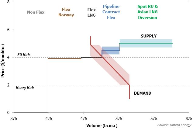
Chart 1 illustrates the current European supply and demand balance using this approach. It is important to note that the chart summarises supply and demand at an annual level. We come back below to some of the important within-year drivers of pricing and flows.

Chart 1: 2016 annual European supply and demand balance

Source: Timera Energy

Supply

The chart shows sources of European gas supply grouped into several key tranches:

Inflexible price taking supply: consisting of (i) pipeline contract ‘take or pay’ volumes (ii) inflexible LNG contract volumes and (iii) domestic production (very low variable cost ). These ‘price taker’ volumes flow regardless of hub price levels.
Norwegian flexible volumes: consisting of Norwegian production flexibility and flexible hub indexed contract volumes. These volumes are also effectively ‘price taking’ given Norway produces to an annual production target, but they are shown at a slight discount to current hub prices to reflect the fact that flows are optimised against hub prices.
Flexible LNG volumes: made up of divertible European LNG supply contract volumes and LNG spot cargoes surplus to the requirement of other regions. Volume and flow depends on netback LNG spot price differentials relative to European hub prices.
Pipeline contract flexibility: from predominantly Russian oil-indexed swing contract volumes above ‘take or pay’ levels.
Spot Russian & incremental LNG: gas volumes that may be induced to flow into European hubs if prices rise sufficiently to attract (i) incremental Russian spot flows and (ii) diversion of LNG from other regions (predominantly Asia where fuel substitution is possible, typically to oil products).

The interaction between tranches 2, 3 and 4 and demand is the place to focus in order to understand price dynamics.

Demand

European gas demand is relatively price unresponsive in the shorter term, except for the power sector. The downward slope of the demand curve in the chart reflects the potential impact of coal to gas plant switching across European power markets as gas prices fall.

The amount of additional gas demand that is generated at lower hub prices depends on relative gas vs coal pricing. But there is 50+ bcm of switching potential if coal prices remain relatively stable while gas hub prices continue to decline towards Henry Hub. We will come back in a subsequent article to explore this dynamic in more detail, but it is going to be a key factor driving gas market dynamics over the next 2-3 years.

Pricing at the margin

Declining hub prices in 2016 are being driven by a battle to place Norwegian flex, LNG imports and Russian pipeline volumes across European hubs. This is in addition to the large volume of ‘must flow’ gas shown at zero price in the chart.

Oil-indexed contracts have historically played an important role in setting hub prices at the margin (the intersection of supply and demand). Oil-indexed prices tend to act as a magnetic force given the use of swing gas to balance the market. But as 2016 progresses into 2017, the impact of the tipping point we foreshadowed this time last year looks set to gather momentum.

A combination of robust production flows (particularly from Norway) and rising LNG imports are pushing oil-indexed contract prices off the margin. The result is that hub prices (currently around 4.00 $/mmbtu) are falling below oil-indexed contract benchmarks (4.50+ $/mmbtu). With hub prices at a discount to contract prices, suppliers are incentivised to reduce contract volumes to take or pay levels.

The damage to hub prices is being caused by increasing volumes of supply being pushed in to the European market to left of the margin. Robust production levels and rising LNG imports are forcing the supply curve down the demand curve to clear the market at a price level which induces an adequate volume of power sector demand response.

For evidence of this look to the UK and Italian power markets. CCGTs are the dominant form of generation in both markets and load factors have increased significantly across the last 6 months as gas prices have fallen. Peak clean spark spreads in other Continental power markets have also recovered, foreshadowing the potential for a much higher volume of switching if hub prices continue to decline.

Within-year dynamics

For the purposes of this article we have shown an annual view of supply and demand to summarise high level drivers of hub pricing. But behind this our analytical framework allows us to drill down into a number of more complex factors that determine how the market clears on a within-year basis. These are worthy of a separate article but we provide a brief summary here to highlight their role:

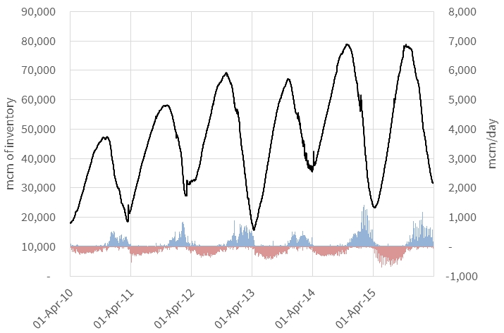
Gas storage plays a key within-year balancing role, both seasonal and to dampen shorter term price volatility. The influence of storage is largely netted out at an annual level (hence its absence in the chart) but it remains a key driver of pricing dynamics at a sub-annual level.
Norwegian production flows have a pronounced seasonal profile (higher in winter) and are optimised by Statoil on a day to day basis across their different hub access delivery points.
Take or pay profiling of oil-indexed contract volumes is driven by the relative relationship between hub and contract prices across the year (with suppliers incentivised to take gas when it is cheapest based on a 6-9 month oil price lag).
LNG imports can ebb and flow into European hubs based on short term fluctuations in global spot prices.
Weather can have a significant influence on gas demand. This was illustrated by very low 2014 gas demand due to unusually mild winter.

While these factors increase the complexity of the supply and demand balance at any point in time, they do not materially erode the relevance of the annual level view shown in Chart 1.

Looking forward, the US market looms large below

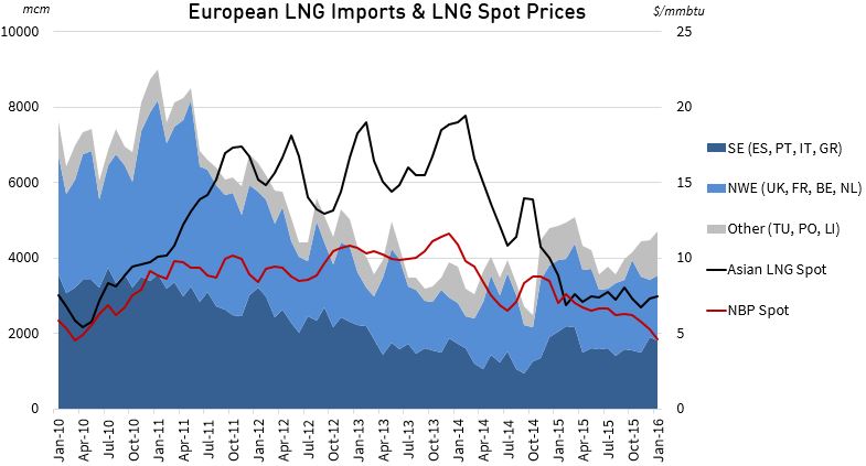
A key unknown variable remaining across the next two years is the level of surplus LNG Europe will need to absorb as new liquefaction projects ramp up production, against what appears so far to be a backdrop of weak Asian demand. There has been a noticeable increase in LNG flow into North West European hubs over the last 12 months as we showed last week. But this volume is small relative to an anticipated 23 bcm ramp up in new LNG flow into the global market across 2016 and 35 bcm in 2017.

There have however been some notable delays in production from new liquefaction projects e.g. Gorgon and Sabine Pass. It should also be recognised that trains often take 6 months or so to achieve 90% of nameplate capacity, so there is a lag to take into account (as well as the ongoing poor performance of some established LNG suppliers).

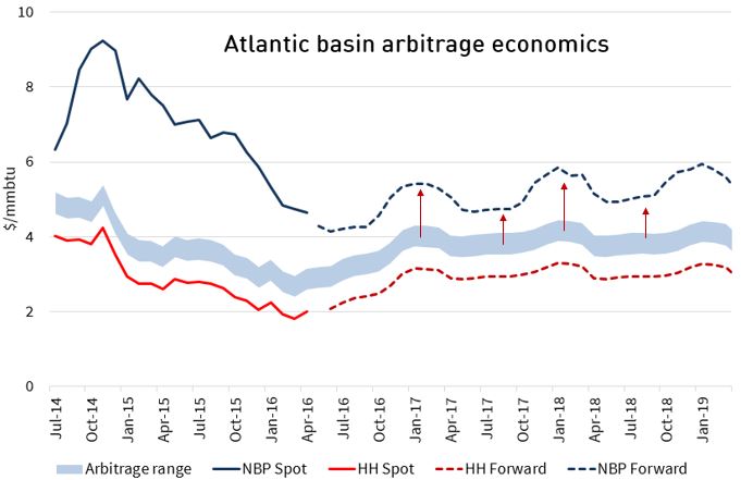
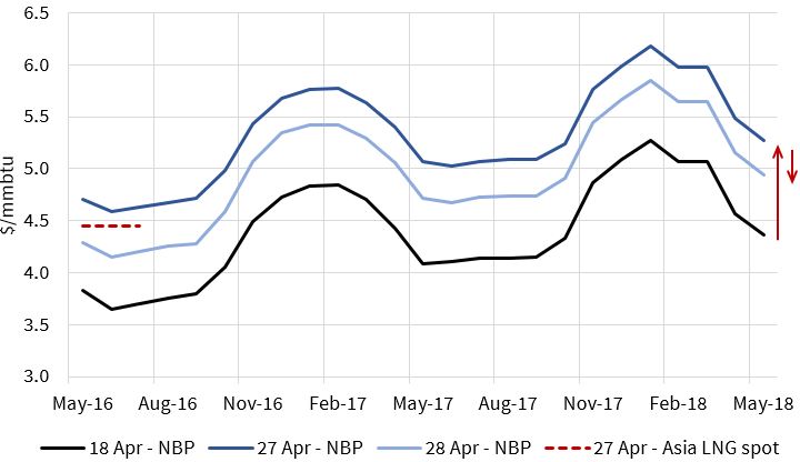
The Asian LNG spot price differential above European hubs is a barometer for how much of this new LNG may flow into Europe. That spread is currently approaching zero. That means Europe is the most attractive place to send surplus cargoes, LNG that as it is absorbed will place downward pressure on hub prices.

This is why we expect coal to gas switching dynamics to attract much more focus as 2016 develops. The importance of the role of switching is not widely understood. As the influence of oil-indexed contract pricing is eroded, the supply side of the European gas market is set to become increasingly dominated by price insensitive volumes of supply (inflexible production, Norwegian flows and LNG imports). This shifts the market focus to demand response and the relative variable costs of CCGTs versus coal generators.

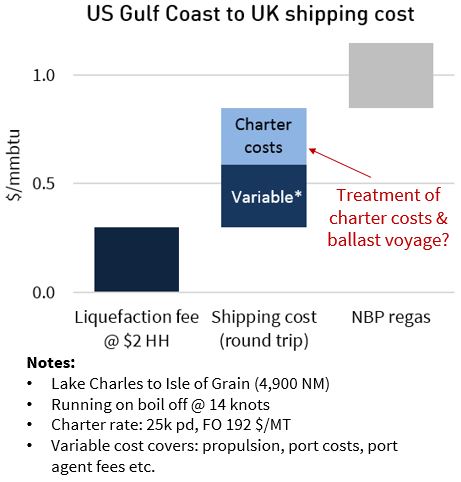
As oversupply increases, the other source of European hub price support comes from across the Atlantic. If hub prices continue to decline, US exports will be ‘shut in’ on a variable cost basis. We estimate shut in to occur at a Henry Hub to NBP/TTF spread between 0.5-0.8 $/mmbtu, the sum of variable liquefaction, shipping and regas costs. The cost range depends on the extent to which off-takers have committed to shipping and regas capacity on a medium/long term contractual basis, in which case it is a ‘fixed’ cost. But regardless of shut in dynamics, US export volumes remain small until 2018.

Beyond coal-gas switching in the power sector, further support for European hub prices could derive from Russia relaxing its contract take or pay levels with European contractual buyers. This would take physical gas ‘out of the system’ and help the market to clear. However if this does not happen it is possible that European hubs could converge with Henry Hub.

In this situation the ultimate source of European hub price support is the diversion of surplus global cargoes to the US market instead of Europe. Don’t laugh … it happened during the last global glut in 2009. In a bitter irony for US exporters, this could mean a period of reemergence of US imports at the same time new US liquefaction capacity is being commissioned.

Article written by David Stokes, Olly Spinks and Howard Rogers

Global LNG and European gas workshop

Timera Energy offers tailored workshops exploring the evolution of the global LNG and European gas market fundamentals and pricing dynamics. These workshops involve Howard Rogers who, as the Director of the Gas Programme at the Oxford Institute for Energy Studies, is acknowledged as a leading industry expert in the global gas market.

If you are interested in more details please email olly.spinks@timera-dev.positive-dedicated.net

European LNG imports on the rise

Posted on April 18, 2016January 16, 2020 by David Duncan

The post-Fukushima Asian LNG price premium saw European LNG imports fall by more than 50% across the 2011 to 14 period. In 2011, the year of the Fukushima disaster, Europe imported 91 bcm of LNG. By 2014 European LNG imports had fallen to 42 bcm, representing a 49 bcm reduction from three years earlier.

Over the same 2011-14 period European gas demand fell 65 bcma. This was predominantly driven by falling power sector demand as CCGTs were displaced by cheaper coal and renewable generators in power market merit orders. Asia’s ability to absorb high volumes of diverted European LNG across this period helped dampen the impact of falling demand.

But stepping forward to 2016, the Asian LNG spot price premium over Europe has all but gone. Asian spot prices have now essentially converged with European hub prices around 4 $/mmbtu. And LNG flows into Europe are increasing again despite an already oversupplied market.

European LNG import evolution

The 2011 Fukushima disaster marked the end of the last period of global oversupply, caused by the parallel effects of the financial crisis and 2008-10 ramp up in liquefaction capacity. Japanese LNG demand jumped (~30 bcma) as nuclear plants closed. At the same time, robust demand growth from developing importers and feed gas constraints for a number of exporters helped tighten LNG market conditions.

Fukushima also marked an inflection point for European LNG imports, as a tightening global market caused a rapid rise in Asian spot LNG prices. The Asian price premium that opened up over European hub prices across 2011-14 had two important effects:

It created a strong incentive for European gas portfolios to flow flexible LNG cargoes to Asia, or to reload cargoes for re-export if contractual conditions precluded diversion
It also created an incentive for European buyers to negotiate greater diversion flexibility into LNG contracts (both existing and new)

The combined impact of these effects was to divert almost 50 bcma of LNG from Europe to Asia across the 2011-14 period. Chart 1 shows the structural decline in LNG imports across this period.

Chart 1: Monthly profile of LNG imports

Source: IEA data (LNG flows), Reuters (Asian spot) & ICE (NBP spot)

2014 marked a major turning point in the global LNG market. The year began with spot prices above 20 $/mmbtu as Asian buyers chased cargoes. But by the end of 2014, Asian prices had crashed to half this level.

October 2014 marked the low point for European LNG imports this decade. However the signs of a turning point for imports were already emerging across the summer of 2014. In order to better illustrate this we have broken European imports down into 3 categories in Chart 1:

Southern Europe: A grouping of regas terminals in less liquid gas markets dominated by Spain.
North West Europe: Terminals connected to Europe’s liquid NBP and TTF hubs.
Other: Terminals on the fringe of the European market which are less responsive to market price signals (Turkey, Poland, Lithuania)

The chart shows a clear recovery in LNG import volumes into NW Europe across the summer of 2014. This coincided with the re-convergence of Asian and European spot prices and a ramp up in surplus cargo volumes sold into Europe’s liquid hubs. Rising LNG imports was one of the factors behind a sharp decline in NBP/TTF hub prices across Summer 2014.

The trend of higher LNG imports into NW Europe has continued through 2015-16 as the global market has tipped into a state of oversupply. At the same time Southern European import volumes have stabilised as the incentive to divert cargoes to Asia has disappeared. The evolution of import volumes over the next three years of rapid supply growth will be a very important driver of European hub price dynamics.

Europe’s evolving role as a gas sink

As 2016 progresses, Europe is set to take on an increasingly important role as the LNG market of last resort. The liquid NW European hubs at NBP and TTF will set the price benchmark for surplus cargoes as LNG export volumes ramp up from new Australian and US liquefaction terminals.

In distance terms it may appear cheaper to flow much of this surplus gas into Mediterranean terminals. But there are two important factors that are likely to keep the focus on NW Europe:

Regas terminal access costs in Southern Europe (particularly Italy) are high relative to NW Europe
Access to liquid forward curves at NBP and TTF provide an ability to hedge the sale of cargoes ahead of delivery

This is good news for regas terminal operators (and terminal value) in NW Europe after what has been a tough period of lower than expected volumes versus those projections used to underpin terminal investment cases.

As imports into NW Europe increase the power sector will again come back into focus. Demand response from gas to coal switching in European power markets is set to play an important role in balancing the European market as hub prices fall. We return next week with a supply and demand balance view of the European gas market to illustrate this and other forces driving price evolution as 2016 progresses.

Article by David Stokes & Olly Spinks

Long term contract pricing: counterparty motivations

Posted on April 11, 2016January 16, 2020 by David Duncan

The pricing terms of long term contracts on flexible gas & power assets are typically the subject of lengthy negotiations. They also often remain a closely guarded commercial secret. This is reflective of the bespoke nature of these contracts and the large sums of money involved.

Long term contracts are used to underwrite investment in a wide range of flexible assets including midstream gas assets (e.g. pipelines, storage facilities and LNG terminals) as well as thermal power plants and electricity interconnectors. Pricing terms vary widely across different asset types and counterparties. But behind the negotiation of individual contract pricing terms there are a set of common principles that apply.

We recently published our first article in a series on the long term contracting of flexible assets. In our second and third articles in this series we focus on the drivers of contract pricing. In today’s article we consider the motivations of the contract sellers and buyers at the negotiating table, in order to understand how these impact the pricing of contracts. We then set out a practical explanation of the 5 key drivers of contract prices in our next article in the series.

Seller motivations

The sellers of long term contracts are typically asset owners. Contract sales may be to support the development of a new asset (e.g. a CCGT tolling deal) or to manage the margin of an existing asset (e.g. sale of pipeline or storage capacity). Either way long term contracts involve the structural transfer of asset exposures from seller to buyer. This means exposure management plays an important role in shaping the motivations of contract sellers.

There are three important factors that drive seller negotiation of contract pricing terms:

Risk tolerance
Return on capital
Route to market

The first two of these factors are intimately related. The seller of a long term contract is principally focused on how pricing terms will impact the risk/return profile of the underlying asset (as we set out in detail here). The contract price level needs to support an adequate return on capital employed. But the pricing structure also needs to deliver that return within a tolerable level of risk.

Take for example a gas storage operator looking to sell long term capacity to support the incremental expansion of a storage facility. Current weakness in market price signals (seasonal spreads and spot volatility) make it challenging to sell long term capacity contracts at a price level that supports investment. In order to increase returns, the storage operator can seller a lower volume of long term contracts (i.e. retain more market risk). Or alternatively they can introduce some degree of market indexation into contract pricing terms (e.g. spread indexation). But either way these decisions impose additional risk on debt and equity capital invested in the project. Seller’s negotiation of contract pricing terms revolves around balancing these risk/return considerations.

Route to market (factor 3. above) only applies to a subset of long term contract negotiations. It relates to using the counterparty (or buyer) to access the commercial capabilities required to monetise asset value (e.g. a trading capability). This is typically only a concern for asset owners that do not have an internal marketing and trading function. But route to market agreements are becoming an increasingly common feature of long term contract negotiations, given the growing importance of infrastructure investors without a market facing capability.

Route to market contract terms typically cover a fixed service fee combined with variable execution fees. These may be negotiated separately from the structural pricing terms of long term contracts. However it is often the case that both pricing and route to market terms are agreed at the same negotiating table with the same counterparty. This means that route to market capability and cost competitiveness can influence a seller’s attitude to contract price terms.

Buyer motivations

While long term contract sellers can typically be characterised as asset owners, there are a number of different types of contract buyers. To understand buyer motivation in negotiating contract pricing terms, it helps to group buyers into four categories:

Portfolio balancing (e.g. system operators)
Portfolio management (e.g. physically focused suppliers)
Asset backed trading desk (e.g. utility or producer trading desks)
Non asset backed trading desk (e.g. commodity trader or bank intermediaries)

Like for sellers, exposure management considerations play an important role in shaping buyer motivations. The characteristics of these buyer types are summarised in Chart 1.

Chart 1: Motivations of different buyer categories

Physically focused buyers

Category 1 and 2 buyers are characterised by risk aversity and a focus on maintaining security of supply. In the case of a system operator this is about contracting adequate levels of flexibility to maintain system integrity. For a physically focused supplier (e.g. a gas distributor) it is about ensuring continuity of service to a customer base. This security of supply focus often means long term contracts are priced on an insurance premium basis rather than a purely commercial basis.

Market focused buyers

Category 3 and 4 buyers consist of trading desks that have a greater risk tolerance and market focus when negotiating contract pricing terms. These buyers typically price contracts based on expected merchant returns. However they apply a haircut (or discount) to merchant value to reflect the costs of monetising contract value in traded markets. We will come back to contract haircuts in our next article, but they are primarily driven by the risk capital costs of associated trading activity.

Different buyer motivations can be illustrated via a long term gas storage contract example. The appetite of a commodity trading company to sign a storage contract is driven by the expected returns that can be made via optimising storage capacity against liquid gas hub prices. A gas distributor on the other hand is driven by a requirement to secure a certain minimum volume of physical storage flexibility within its portfolio in order to maintain security of supply to its residential customer base. This decision is driven by the costs of alternative sources of flexibility rather than the value of optimising storage capacity against the market.

Buyer and seller interaction to determine contract price

The pricing terms of a long term contract need to align the interests of the contract seller and buyer. This means satisfying the risk/return (and potentially route to market) requirements of the seller. And doing so with a pricing structure that offers value to the buyer.

This process is usually facilitated by the exchange of draft term sheets between the sellers and prospective buyers to narrow down potential counterparties. Pricing terms are only one of many points of negotiation. But they are typically the most important.

Differences in buyer motivation often lead to confusion as to whether long term contract prices are driven by merchant returns or insurance premium dynamics. The answer is often both.

Merchant returns, adjusted for an appropriate haircut, provide a base level of support for contract prices. This is because there are a range of counterparties competing to access margin from the commercial optimisation of contractual flexibility. These include commodity trading companies (e.g. Danske Commodities, Mercuria, Trailstone) as well as asset backed traders (e.g. RWE Trading, BP, Statoil).

However physically focused buyers may pay a higher price for contracts than that implied by merchant returns, if driven to do so by portfolio security of supply or risk management requirements. Take for example a transmission operator that needs access to physical gas storage flexibility to support system balancing. The extent of the insurance premium the system operator is prepared to pay comes down to the availability of alternative sources of flexibility (e.g. other storage capacity, line pack, production swing).

And this is where there is typically a circularity back to market driven returns. As European energy markets evolve, differences in the pricing of gas and power flexibility across asset types are increasingly being arbitraged away via access to liquid markets.

Article written by David Stokes, Olly Spinks

Summer gas price pressure & the storage overhang

Posted on April 4, 2016January 16, 2020 by David Duncan

Gas storage facilities have traditionally been the seasonal balancing force in the European gas market. Across the EU-28 countries there is around 90 bcm of gas storage capacity, supporting an inventory of approximately 20% of total gas demand.

The first week of April marks the start of the storage year. This is typically the point in the annual storage cycle when facilities switch from winter withdrawal (at higher winter prices) to injection (at lower summer prices). This year European storage facilities are holding an unusually high inventory into the start of the storage year. This will contribute to downward pressure on European hub prices over the summer.

European storage volume and price dynamics

Gas Infrastructure Europe publishes daily updates of storage inventories, injection and withdrawals across the EU-28 countries. While the data is not perfect it gives a useful overview of storage trends. Chart 1 shows the evolution of inventories and flows this decade.

Chart 1: EU-28 storage inventory, injection and withdrawal data

Source: Timera Energy (GIE data)

The increasing inventory over time is partially driven by new and existing facilities being added to the GIE database. The chart shows current storage inventories (32 bcm) are around 30% higher than at the start of the 2015-16 storage year 12 months ago (24 bcm). In 2016 Europe is set to carry the highest storage inventory into summer so far this decade, excluding summer 2014 (when the first down leg of the current global gas price slump occurred).

There have been two main drivers of a high storage inventory into summer 2016. On the demand side it has been another relatively mild winter curtailing gas consumption. On the supply side production flows have been higher than expected over the winter, particularly from Norwegian fields.

Storage capacity holders are also suffering from very weak market price signals. The key market signal that drives storage injection and withdrawal is the summer/winter price spread. The seasonal spread at European hubs is currently at historically low levels as shown for TTF in Chart 2.

Chart 2: TTF summer/winter price spreads

Source: Timera Energy (LEBA data)

With a weak seasonal spread price signal, the focus of storage traders shifts to optimising against shorter term fluctuations in prices (i.e. spot price volatility becomes more important). As winter draws to a close, the price differential between the day-ahead and forward hub prices becomes an important driver of storage withdrawal decisions and inventory draw down. Gas is typically withdrawn as long as the spread between the day-ahead and summer contract prices remains positive (allowing for gas transport & transactions costs). But day-ahead prices have remained relatively weak across Q1 given benign market conditions. That has led to lower withdrawal rates and a higher storage inventory level than normal.

Roll on the summer

Buying gas to inject into storage is a key driver of summer demand at European gas hubs. Higher levels of storage inventory into summer 2016 mean that there is likely to be around 7bcm less demand for injection this summer than there was last year. That adds to downward price pressure at European hubs. There are two other important factors that come into play over the summer that will likely reinforce this price pressure.

Firstly the slump in oil prices at the start of 2016 is going to start to feed through into oil-indexed contract prices across the summer. This means cheaper pipeline gas imports and an incentive for suppliers to profile their volume take accordingly.

Secondly European absorption of surplus LNG cargoes is set to increase as the year progresses. The huge Gorgon LNG project in Australia has just shipped its first LNG cargo. Gorgon production joins the ramp up of the 3 Gladstone LNG projects in Queensland and Sabine Pass in the US.

The combination of these factors will be an important test for the resilience of European gas hubs as the summer progresses. Front month NBP & TTF prices fell below 4 $/mmbtu last week, helped by a weakening pound. That means the spot spread of NBP/TTF over Henry Hub has narrowed to around 2 $/mmbtu. Watch for that gap to narrow further as the year progresses.

Article written by David Stokes & Olly Spinks.

A revival in contracting of flexible assets

Posted on March 21, 2016January 16, 2020 by David Duncan

Long term contracts are a cornerstone of the energy industry. They play a key role in underpinning the capital expenditure required to develop assets. They also play an important role in ensuring security of supply.

There is a long history of contracting gas and power assets in Europe. The role of long term contracts has evolved with market conditions, availability of capital and changes in industry business models. This is particularly true for the contracting of flexible assets such as thermal power plants, interconnectors, pipelines and gas storage facilities, which typically involve the management of significant market risk exposures.

Long term contracts played a pivotal role in facilitating the development and acquisition of flexible assets through the early stages of European gas and power market liberalisation in the 1990s. The landscape then changed in the post Enron bust period of the early 2000s. A strong push for scale and vertical integration saw European utilities internalise flexible asset exposures within their portfolios. This has led to somewhat of a decline in the role and availability of long term contracts over the last decade.

But three factors are currently driving a resurgence in the contracting of flexible assets in Europe:

Balance sheet weakness is increasing pressure on utilities & producers to divest flexible gas and power assets (E.ON and Vattenfall being two prominent recent examples).
Cash rich infrastructure and private equity funds are looking to acquire these assets, but to outsource the majority of market risk via long term contracts in order to protect equity and avoid the overheads associated with setting up internal trading capabilities.
More willing lenders are offering attractive financing terms given low interest rates and a hunt for yield, but are seeking long term contract protection to ensure adequate cashflow stability.

As a result of these factors we have seen a surge in activity to structure & value long term contracts on flexible assets over the last 12-18 months. Available contract terms are asset specific, depending on factors such as the level of intrinsic margin and underlying market conditions. But there are some key practical principles that apply more generally for the contracting flexible assets. Today’s article is the first in a series of articles that sets out these principles, using case study examples to illustrate how they work in practice.

Asset contracting is a risk/return decision

Any sensible consideration of long term contracting revolves around a risk/return decision. This means the risk appetite of the asset owner is usually the starting point for defining an appropriate contracting structure. Contract impact on asset risk is driven by three main attributes:

Volume: the portion of an asset margin that are covered via contract
Duration: the time horizon over which margin is contracted
Price: the contract pricing terms in relation to the asset’s underlying market exposures e.g. fixed, collared, indexed

These terms can vary considerably across contracts. But a set of principles on risk/return apply across all contract structures.

Consider the development of a new UK CCGT plant as an illustrative case study. Let’s assume the majority of capacity of the CCGT is contracted via a fixed price (annual capacity fee based) tolling contract. Chart 1 shows a simplified diagram of the impact of the contract on annual asset gross margins.

Chart 1: Contracted vs uncontracted asset margin distributions (UK CCGT example)

Source: Timera Energy

The blue line shows the frequency distribution of uncontracted (or merchant) asset gross margins. This distribution is relatively wide given the asset is fully exposed to market risk (i.e. to the market sparkspread). The black line shows the distribution of asset margins with the tolling contract in place. It should be noted that the distributions in the diagram are illustrative. In reality these will be driven by the relationship between a specific set of contract terms and underlying market price distributions.

The difference between the uncontracted and contracted distributions illustrates the main principles of asset contracting:

Risk: Contracting reduces the variance of the distribution of asset margins, restricting downside but also limiting upside. In other words it reduces the owner’s risk of margin outcomes deviating from expected levels. For the CCGT asset example, the tolling contract acts to lock in a fixed capacity fee on a portion of asset flexibility value, reducing exposure to the market sparkspread.
Return: There is no free lunch. Contracting also acts to reduce the expected level of annual asset margins. This is because the counterparty on the other side of the contract is forced to take on market risk and needs to be appropriately compensated to do so. In other words the counterparty applies a haircut (or discount) to expected margin levels. Quantification of this contract haircut is driven by factors such as market volatility, asset ‘in the moneyness’ and contract duration, which determine the risk capital required by the counterparty to support the contract.

There are many other considerations involved in successfully executing a long term contract. But understanding the risk/return impact of contracting is an important place to start. This is not a qualitative exercise, it requires numbers.

In other words it relies on the practical quantification of the impact of contracting on asset risk/return distributions. A failure to realistically quantify contracted project economics in advance of securing a capacity agreement has been one of the major road blocks that has stalled the Trafford CCGT development project in the UK.

Contracting to protect equity and debt

Equity investors in flexible gas and power assets can face a tough challenge in defining and securing appropriate volume, duration and pricing terms. The level of intrinsic margin or ‘in the moneyness’ of an asset is an important factor determining whether contracting makes sense. It is also a key factor determining lender willingness to provide debt.

This can be illustrated by looking at some examples of assets with different margin structures:

Deep in the money: The interconnector assets that are being developed between Continental and the UK power markets benefit from high structural intrinsic margins. Forward power prices in the UK are currently at more than a 15 €/MWh premium to France and Belgium. Margin stability associated with the ‘in the moneyness’ of interconnector optionality acts to reduce long term contract price haircuts. It also means a greater portion of asset cashflow can be contracted to protect equity returns and secure debt.
Less in the money: A broad range of flexible European assets currently have some structural margin, but at levels that make contracting a challenge. These include gas pipeline, gas storage and some thermal power assets (e.g. UK CCGTs). The defining factor for a successful contracting strategy is ensuring that the associated reduction in risk adequately compensates for the reduction in asset return. This can be very difficult when contract buyers, typically energy trading desks, heftily discount contract prices to reflect the risks associated with a lack of intrinsic margin.
At or out of the money: If an asset has little or no intrinsic margin (e.g. thermal power assets in Continental Europe) then contracting typically makes no sense. This is because the return on these assets is driven by extrinsic value associated with market volatility or structural market recovery. Realising this value usually means adopting a merchant strategy rather than locking in weak returns via a long term contract.

Chart 2 illustrates some of the issues involved by returning to the UK CCGT tolling example. Expected asset return is the difference between expected gross margin (at the centre of the margin distribution) and the costs associated with plant opex and any debt servicing (shown via the grey and red bars respectively).

Chart 2: Structure of contracted asset return (UK CCGT example)

Source: Timera Energy

The merchant or uncontracted margin distribution (in blue) shows a significant risk of margin falling short of plant opex and debt service costs (i.e. distribution downside exposes debt/opex levels). Contracting acts to:

Reduce downside risk shifting the tail of the cashflow distribution to the right and reducing the probability that margin falls short of debt service and opex costs.
Reduce expected return moving the expected plant margin down from the blue dashed line (uncontracted) to the black dotted line (contracted) and reducing the level of asset return above costs.

Defining a contract structure that balances these requirements becomes more difficult the lower the intrinsic margin or ‘in the moneyness’ of the asset. This in a nutshell is the challenge facing European investors looking at flexible gas and power assets.

An investment and contracting case needs to be built around providing adequate downside protection for equity and any debt. But at the same time ensuring that an adequate expected return on equity can be maintained. This challenge is not an easy one to overcome given the decline in intrinsic margin of many assets. But it is driving the innovative evolution of both contracting and financing structures, a topic we will return to in our next article in this series.

The blog will take a one week break for Easter but we will be back on April 4th.

Article written by David Stokes & Olly Spinks

Fixing the UK’s broken capacity market?

Posted on March 14, 2016January 16, 2020 by David Duncan

What do you do if you design a capacity market that doesn’t work? Try, try again. The imminent threat of large volumes of coal plant closures has sent DECC rushing back to the drawing board.

This month a raft of proposed revisions to the UK capacity market have been announced for consultation. It is DECCs intention to implement these changes by the summer, in time for the start of the 2016 capacity auction process.

DECC is now fighting a security of supply battle on two fronts:

Closure prevention: To ensure enough existing capacity remains on the system during the capacity crunch over the remainder of this decade
New build: To incentivise the delivery of large scale new capacity into next decade to replace closing thermal plant

This was reflected in the UK energy secretary’s accompanying statements:

“By buying more capacity earlier we will protect consumers and businesses from avoidable spikes in energy costs”

“We’re also sending a clear signal to investors that will encourage the secure and clean energy sources we need to come forward, such as gas and interconnectors”

The first statement would have made more sense three years ago when DECC first implemented the capacity market. The second statement reflects DECC’s barely disguised preference for CCGTs and interconnectors as a new build solution.

DECC’s proposed revisions to the Capacity Market reflect its security of supply concerns. These are focused around two main measures:

Early implementation: Pulling forward the capacity market a year via a new capacity auction to be held in Jan 2017 in order to remunerate plants in 2017-18
Buying more capacity: Increasing the capacity target level in this year’s T-4 auction, to increase capacity in the 2021-22 delivery year

In this article we look at what these measures mean for the UK power market.

Early implementation (2017-18)

DECC’s early implementation measure is all about keeping existing capacity on the system. The 15 year capacity agreements, used to incentivise new build in previous auctions, are not available in the 2017-18 auction. Given the short delivery lead time of 9 months there are only 1 year capacity agreements on offer.

This measure will in effect replace the much criticised Supplemental Balancing Reserve (SBR) mechanism that is currently being used to maintain UK security of supply. The removal of SBR is long overdue given it has become increasingly unpopular and unruly over the last two years.

Plant closure announcements have forced National Grid (the TSO) to buy more and more ‘emergency reserve’ capacity to protect security of supply. Table 1 provides a summary of the 3.5 GW of SBR capacity Grid have purchased for Winter 2016-17.

Table 1: Winter 2016-17 SBR plants and volumes contracted by National Grid

Source: National Grid

This table reads like a power plant endangered species list. The SBR capacity was procured for a total cost of £122m at an average price of 34 £/kW, 70% higher than capacity clearing prices in the first two T-4 auctions. Individual units were paid up to 88 £/kW for capacity.

SBR payments of this magnitude represent a glowing incentive for existing plants (particularly less efficient coal), to make closure announcements and bid for lucrative SBR contracts. This dynamic has forced DECCs hand in replacing SBR with something more consistent with the official capacity market.

While the removal of SBR is a positive step, the 2017-18 early implementation measures smell of panic. Running a capacity auction for one year agreements at such short notice will likely achieve DECC’s aim of driving up the capacity price. But it will do so at a substantial cost to the consumer.

The supply curve in the 2017-18 auction will be much steeper than normal given a reduced range of capacity options to meet the target. Existing coal plants are likely to be an important driver of clearing price. Coal plants will need capacity payments to cover station fixed costs (~40-50 £/kW), less any dark spread margins and delayed closure cost benefits, in order to remain open for the next two winters.

Say for example the 2017-18 auction clears at 35 £/kW with the government procuring 50GW of capacity (these are illustrative round numbers). This would cost the consumer £1.75bn. This is more than 14 times Grid’s cost of procuring SBR capacity for Winter 2016-17 (£122m). In other words the auction represents a huge windfall to existing plants that are going to remain open anyway.

Beyond this 2017-18 ‘one off’ auction, DECC will need to purchase incremental capacity in the T-1 auctions to ensure security of supply (given the absence of SBR). The supply curve for these auctions is likely to be steep and clearing prices higher for similar reasons to those described above i.e. limited competition to provide incremental capacity at short notice. Structurally higher T-1 capacity returns over the next 5 years is something to start factoring in to asset investment decisions. But these higher prices will only accrue to plants that do not already have contracts from the T-4 auction.

Buying more capacity (2021-22)

Leaving to one side the problem of security of supply over the next 5 winters, DECC is also rightly focusing on next decade. To give credit where it is due DECC appears to be taking a more sensible approach to the new build issue. Suggestions of introducing an entirely new set of interventions to support CCGT new build appear to have been shelved.

Instead DECC is focusing on using the existing Capacity Market but raising the capacity target level. DECC has provided guidance that 2021-22 target demand levels will be at least 3GW higher than would normally be the case. DECC’s intention in doing this is primarily to incentivise gas plant new build. But it will not necessarily result in new CCGTs being delivered.

We estimate a new CCGT project to require a minimum of 40-45 £/kW (via a 15 year contract) to proceed, given current available terms on tolling contracts and financing. The new penalties for non-delivery of capacity that DECC intends to introduce if anything act to increase the required capacity price.

Whether the clearing price in this year’s T-4 auction reaches these levels will depend on the steepness of the supply curve. But we suspect that capacity price levels between 20 and 40 £/kW will start to flush out large volumes of alternatives to CCGT capacity.

DECC will likely ensure that the use of higher emissions diesel generators is restricted via appropriate emissions legislation. It would be a mistake to do this via heavy handed fiddling with embedded generation benefits. But we suspect gas-fired peakers and an interesting range of other alternative supply sources may become apparent as capacity prices rise.

This is after all what the capacity market should be about. Competition to provide the cheapest form of incremental capacity, not a blunt instrument with which policy makers try and pick winners.

Article written by David Stokes and Olly Spinks

Rising CCGT load factors and gas volatility

Posted on March 7, 2016January 16, 2020 by David Duncan

The sharp decline in gas hub prices in 2016 is starting to reshape the landscape for flexible supply infrastructure in European gas and power markets. CCGT load factors are on the rise as coal plants are being displaced from the merit order. Spot gas price volatility is also showing early signs of recovery despite an oversupplied European gas market.

2016 may mark the start of an evolving relationship between CCGT load factors and gas price volatility. Falling CCGT load factors have been the main driver of the slump in European gas demand this decade. So increasing gas plant competitiveness is starting to support a recovery in power sector gas demand.

In addition as gas prices fall CCGTs play a more prominent role in setting marginal power prices. This means CCGTs provide more of the marginal flexibility required to back up short term swings in intermittent renewable output. So swings in CCGT gas demand are in turn supportive of higher prompt gas price volatility.

In today’s article we explore whether a recovery in CCGT load factors across Europe could support a more structural recovery in gas price volatility.

The UK leading a 2016 CCGT recovery

As gas hub prices fall, CCGT load factors are increasing significantly in 2016 versus last year. This is particularly the case in markets where gas plants play a more important role in setting marginal prices e.g. in the UK and Italy.

We like to focus on the UK power market as a barometer for gas vs coal switching in Europe. It plays the role of ‘canary in the coal mine’ for increasing gas plant competitiveness given:

The dominance of CCGT plants in setting power prices
The UK carbon price floor policy that acts to disadvantage coal plants

Chart 1 provides a snapshot of gas vs coal plant competitiveness in the UK power market based on current forward curve pricing for power, gas, coal and carbon. A few notes on the chart:

The chart shows different combinations of gas (vertical axis) and coal (horizontal axis) prices
The coloured dots show current forward curve combinations of gas and coal prices for different seasonal forward contracts from 2016-18
The sloping lines mark the gas vs coal switching boundaries between CCGT plants with different efficiencies (47%, 49% and 52% HHV efficiency) and coal plants (with 36% efficiency)
When a coloured dot sits below the gas vs coal switching boundary it means over that time horizon, CCGTs are displacing coal plant in the merit order (at current forward prices)

Chart 1: Gas vs coal switching boundaries in the UK power market

Source: Timera Energy

The chart shows the UK’s top tranche of newer CCGTs (@52% efficiency) displacing coal plants (@36% efficiency) to run baseload. The second tranche of CCGTs (@49% efficiency) are also displacing coal plants in summer periods. The third tranche of CCGTs (@47% efficiency and below) are providing peaking flexibility.

Falling gas prices are pointing towards the majority of the UK CCGT fleet coming back into merit during summer 2016. The impact of this CCGT displacement of coal plants is likely to be a materially higher UK gas demand in 2016.

The effect of lower gas prices on CCGT load factors is not isolated to the UK. Baseload spark spreads have also been positive in Italy this winter (partly due to relatively low hydro levels), causing a step up in CCGT load factors. Despite mild and windy weather in North-West Europe, there has also been a recovery in gas plant load factors in markets such as France, Belgium and the Netherlands (although baseload spark spreads remain in negative territory).

But gas vs coal switching is still an evolving story in Europe. Hub prices remain under heavy pressure into the coming summer. European gas storage inventories remain at unseasonably high levels into the spring, which will reduce gas demand for storage injection over the summer. European hubs also face a ramp up in LNG imports as Asian spot prices have again slumped under 5 $/mmbtu. These factors point to higher CCGT load factors and gas demand as the year progresses.

Why this is important for gas flexibility value

CCGT load factors form an important source of demand for gas flexibility services. Falling CCGT load factors across the first half of this decade have been the primary cause of an almost 20% fall in European gas demand. The decline in power sector gas demand has contributed to a slump in spot gas price volatility, the market price signal for gas supply flexibility.

A recovery in CCGT load factors across Europe should support spot gas price volatility and the value of supply flexibility. This is particularly true for the rapid response gas deliverability required to support sharp swings in CCGT load factors (e.g. from fast cycle storage).

CCGTs are a key transmission mechanism for prompt price volatility from the power to the gas market. As CCGTs come back into merit, gas swing demand rises to support the ramping up and down of CCGTs in response to shorter term swings in market conditions.

The role of CCGTs in providing flexibility is also set to be supported by the closure of many of Europe’s less efficient coal plants over the next five years. Lower gas prices are rapidly eroding coal plant margins to levels below plant fixed costs. This will be reinforced by German nuclear plant closures early next decade.

Uncertainty remains around the timing and pace of an increase in spot gas price volatility and the value of supply flexibility. But watch for a resurgence in CCGT load factors as an indicator of the start of a structural recovery.

Article written by David Stokes, Olly Spinks & Emilio Viudez

Brent crash in animation (Part II)

Posted on February 29, 2016January 16, 2020 by David Duncan

The wild ride continues in the crude market. Brent plunged below 30 $/bbl earlier this month as resilient production and inventory build spooked the market. This was followed by a sharp 20% rally triggered by the optimistic concept of coordinated OPEC/Russian production cuts.

Any hope of cooperation between Saudi Arabia, Iran and Iraq fell apart last week, with crude falling 5% in a day. But prices snapped back after better than expected gasoline inventory data. The oil market is being whipped about by short term news flow.

Much of this would appear to be of little relevance to longer term prices. But the crude forward curve is also gyrating wildly with fluctuations in spot prices. The crude curve deserves more attention than it gets. For a meaningful bottom to form in the crude market, the US production investment cycle needs to be disrupted. And forward prices are a key benchmark driving the investment decisions of US shale producers.

In this article we return to an updated view of our animation of spot vs crude curve evolution for clues on the evolution of crude pricing dynamics. We also take a look at the behaviour of implied volatility levels in relation to underlying prices.

Back to the movies

We published our first animation of Brent curve evolution in Feb 2015. Chart 1 shows an updated view of the animation a year on.

Chart 1: Brent spot versus forward curve evolution (2008-16)

Source: Timera Energy, ICE data

Perhaps the most striking observation from Chart 1 is the strong relationship between spot prices and the forward curve. But some other interesting dynamics can be observed by focusing in on the back end of the curve:

Financial crisis shock (2008-09): Although spot prices fell below 40 $/bbl, the back of the curve remained above 65 $/bbl.
Recovery (2009-13): The back of the curve was anchored in an 80-100 $/bbl range (driven by production LRMC benchmarks), despite spot prices moving in a much wider band.
Oversupply down leg 1 (2014-15): Spot prices plunged under 50 $/bbl in early 2015, but the back end of the curve remained above 75 $/bbl (again held up by production LRMC benchmarks).
Oversupply down leg 2 (2016- ): In 2016, the back end of the curve has fallen below 50 $/bbl, significantly lower than previous periods of low spot prices.

Oversupply remains pronounced in the short term, with a large global inventory overhang. But in 2016 the forward curve is at levels that do not support new investment in US shale. In other words forward prices are below the Long Run Marginal Cost of shale production (let alone other supply sources). This is illustrated by an ongoing decline in the US rig count. These conditions are supportive of a market bottom and price recovery, even if there may be further short term weakness in spot prices.

There are two other important factors to watch for clues on a market bottom:

A weakening in the US Dollar, given the negative correlation between oil and the USD
Extreme levels of implied volatility in the crude options market

Chart 2 shows the evolution of the CBOE 30 day implied volatility index (OVX) over the same 2008-16 period as Chart 1.

Chart 2: CBOE OVX crude oil volatility index

Source: Timera Energy, CBOE data

It can be seen from Chart 2 that major market turning points coincide with peaks in implied volatility:

Financial crisis low (2008): A peak in the OVX implied volatility index above 100 coincided with the post financial crisis low below 40 $/bbl in late 2008
Recovery top (2011): Another peak above 60 occurred in the OVX at around the time Brent spiked above 125 $/bbl in 2011.
Interim low (2015): The OVX again breeched 60 as Brent formed a temporary bottom below 50 $/bbl in early 2015.

The logic is fairly simple. Market trends tend to reverse during periods of extreme sentiment and uncertainty. This is reflected by high premiums being paid for protection via the options market causing a spike in implied volatility.

Early in February, the OVX spiked towards 80 indicating another period of extreme implied volatility. This does not preclude volatility moving higher still (e.g. towards 100 as in 2008). But it does suggest that the crude market could be in the process of forming a major low.

Article written by David Stokes, Olly Spinks and Emilio Viudez