Utility asset sales: where are the value opportunities?

The article below is our last before the summer break.  We will be back with more in late August.

Three weeks ago we set out the case for an unprecedented sale of conventional supply assets by European utilities. French and Italian utilities alone have announced their intention to sell upwards of €30 bn of assets. And this is only part of a larger pool of assets earmarked for sale across Europe, as utilities & producers shift their strategic direction and respond to balance sheet constraints.

The sheer scale of asset sales should open up substantial value opportunities, as well as paving the way for new entrants. Value is supported by a lack of utility buyers and cyclically depressed conditions in some markets. But potential buyers face the challenge of finding & pricing undervalued assets, while avoiding assets that are in terminal value decline.

In this week’s article we set out our view on two specific value opportunities:

  1. Gas-fired power assets
  2. Mid-stream gas assets

We focus on these because we see structural market changes that support value and offer asymmetric upside. But a robust investment case does not need to be based around a bet on a broader recovery in asset values. Ultimately value creation comes down to buying well chosen assets that are play a structural role in market operation… at the right price.

Value opportunity 1: Gas-fired power assets

European gas plant values have been decimated this decade. This has happened against a backdrop of general overcapacity in European power markets, caused largely by post financial crisis weakness in power demand growth and capacity overbuild. But beyond this, gas plants load factors and margins have suffered specifically from:

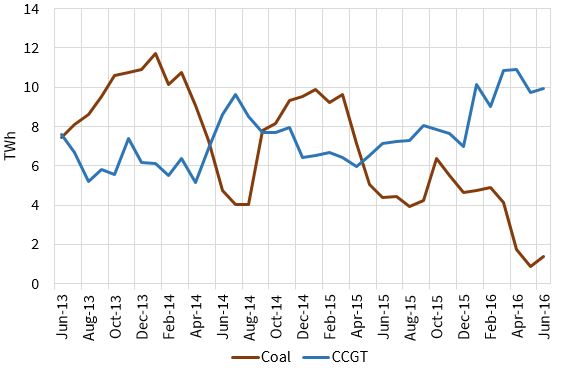
  1. Renewables: The erosion of load factors & prices by rising low variable cost renewable generation
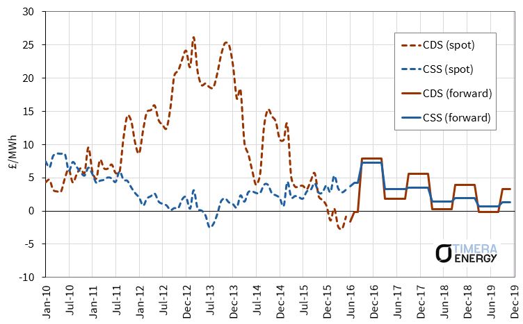
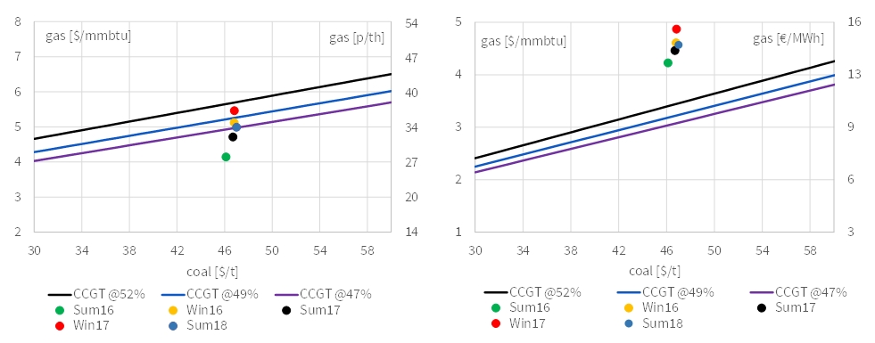
  2. Cheap coal & carbon: Relatively weak coal and carbon prices have favoured coal plant competitiveness over gas plants.

The consensus view amongst utilities is for more of the same. But this ignores some key structural drivers that support a recovery in gas plant load factors, summarised in Table 1 below.

Table 1: Value thesis on European gas-fired power plants

Asset class: Gas-fired power assets
Asset types: CCGT, CHP, gas peaking plants
Status quo: Load factors, margins and asset value have been eroded by cheap coal, increasing renewable output and low carbon prices.
Value thesis:
  • Capacity payment mechanisms are being implemented across European power markets to stem the closure of flexible thermal assets required to back up intermittency.
  • Other revenue streams such as balancing and ancillary services payments are increasing as renewable growth creates transmission systems stress. CHP revenue streams can also provide downside protection.
  • Gas plant competiveness is increasing as gas prices fall (relative to coal prices) in a structurally oversupplied global gas market. Carbon price support may help this.
  • Rising gas plant load factors, margins and new build are set to be a feature of the early-mid 2020s given regulatory intervention to close large volumes of coal and nuclear plant.
Sellers: Potential buyers:
European utilities Funds (infra, PE), smaller utilities/producers


Case study: Continental CCGT assets:

CCGTs in Continental European power markets are widely regarded as value toxic. In many cases this is justified. A number of older, less flexible and/or locationally disadvantaged gas-fired assets are ripe for closure. Even owners of brand new merchant CCGTs in markets such as Germany and the Netherlands are suffering from several years of negative cashflows. Buying assets like this based on the thesis of a sparkspread recovery in the 2020s takes quite a specialised investor risk/return profile.

To build a more stable investment case it is important to target assets that have access to revenue streams that can ‘top up’ wholesale energy margin to cover fixed costs. This incremental revenue can come in the form of capacity payments, balancing & ancillaries revenue or pre-contracted revenue streams (e.g. CHP steam and onsite power contracts). There are also structural factors protecting plant energy margins in some markets e.g. the price setting dominance of CCGTs in UK and Italy and the requirement for gas-fired peaking capacity in Belgium and France.

But covering fixed costs is about buying time for value recovery. There are three important structural shifts taking place that support value upside:

  1. Capacity payment mechanisms are in the process of being implemented across Europe, adding an additional source of revenue that should rise as market capacity balances tighten.
  2. Regulatory driven closures of large volumes of coal and nuclear plants across Europe should increase gas plant load factors and margins in the early to mid 2020s. A number of existing newer/flexible CCGTs are set to become key for security of supply as this happens.
  3. Gas plant competitiveness is improving again as the global market transitions into a period of structural oversupply and gas prices fall. This may be further supported by actions to increase the EU carbon price signal (e.g. the French proposal to implement a carbon price floor).

Relatively new assets that will be critical for security of supply in the 2020s can be bought for a fraction of new build cost (e.g. 15-20%). But the premium that owners pay for access to value upside includes plant fixed costs. The challenge in buying Continental CCGTs is ensuring protection from negative cashflows, while understanding and pricing the risk/return distribution of assets.

Value opportunity 2: Midstream gas assets

The value of midstream gas assets (e.g. pipelines, gas storage & LNG regas terminals) has also suffered this decade. Weak gas demand has been a big factor behind this, particularly as a result of declining CCGT load factors (for the reasons set out above). There are two key price signals for midstream supply flexibility value:

  1. Price spreads: the signal for the value of supply flexibility e.g. seasonal spreads for storage, locational spreads for pipelines.
  2. Prompt price volatility: the signal for the prompt deliverability of gas e.g. in response to demand swings or supply disruptions.

Both price signals have declined to historically low levels this decade, falling from levels that support investment in new gas storage assets, to levels that are forcing the mothballing and closure of existing flexible assets. The consensus view among utilities is again for a continuation of current market conditions.

Table 2: Value thesis on European midstream gas assets

Asset class: Midstream gas assets
Asset types: Gas storage, gas pipelines, LNG regas terminals
Status quo: Asset pricing reflects current historically weak market price signals for gas supply flexibility (price spreads and price volatility).
Value thesis:
  • Import dependency is increasing as European domestic gas production declines, increasing Europe’s reliance on Russian gas (political risk) and LNG imports.
  • Renewable intermittency is supporting gas swing demand as renewable output rises and gas-fired power plants are increasingly required to provide flexible backup.
  • Ageing infrastructure is resulting in the retirement of flexible infrastructure as owners cannot justify investing in life renewal capex.
  • Low fixed costs help support positive cashflows and protect value downside.
  • Asset utilisation is increasing supported by import dependency.
  • Other value support can often be found (e.g. via legacy contracts for pipelines or financing/structuring opportunities around cushion gas for storage assets).
Sellers: Potential buyers:
European gas utilities; oil and gas producers Funds (infra, PE), producers, LNG players


Case study: Faster cycle gas storage assets:

 Midstream gas assets have traditionally sat in utility portfolios. But as utilities refocus strategy and sell supply assets, the midstream transaction flow is increasing.

The value upside story for midstream gas assets is driven by a structural transition in the European gas market. As domestic gas production declines, Europe is becoming increasingly reliant on importing gas from outside its borders (e.g. via LNG and Russian gas), creating an associated midstream flexibility requirement. A growing requirement for gas-fired plants to backup renewable intermittency is also set to flow through into higher demand for gas supply flexibility.

This is happening against a backdrop of ageing infrastructure. An estimated 5% of European storage capacity has been closed this decade. The future of a number of other storage facilities is threatened by market price signals that do not cover renewal capex costs (most prominently the large Rough storage facility in the UK).

A feature of midstream assets that makes them attractive to investors is low fixed costs. The overheads and maintenance costs for pipelines and storage assets are typically a fraction of those for power plants. This means that good assets (e.g. that play a structural role in supporting security of supply or portfolio risk management) are likely to retain positive cashflow as owners wait for value recovery.

Challenges in getting the deal done

 In a low yield investment environment, infrastructure investors are increasingly interested in European energy assets. The investment thesis around some asset classes has attracted a widening interest, with asset pricing starting to reflect this (e.g. UK CCGTs and peakers which we have written about now for several years).

However other classes of assets in the utilities sales queue are less well understood e.g. Continental CCGTs and midstream supply assets. In our view these may now offer better value and more competitive transactions price opportunities. But there are three key challenges in building a watertight investment case.

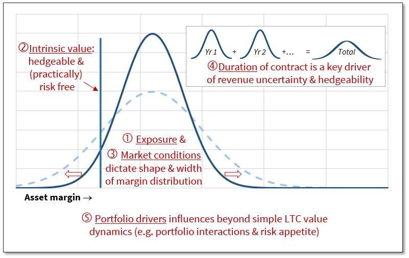
The first challenge is finding some form of downside protection to cover asset fixed costs, while maximising access to value upside (ideally of the asymmetric variety). Upside does not need to be a bet on a broader market recovery but can be built around specific asset benefits (e.g. location, flexibility or barriers to competition). The assessment of the ‘tail value’ of asset margin distributions plays an important role here.

The second challenge is quantifying asset risk/return distributions in order to define a risk adjusted valuation. A robust valuation is built on an understanding of the interaction between the risk/return dynamics of different revenue streams. Infrastructure investors are likely to feature strongly as potential buyers (albeit in partnership with utilities/producers as offtake counterparties). This fragmentation in ownership is likely to require new contracting and business models to support value monetisation and asset operation.

The third challenge is transaction price, given asset value is ultimately a function of price paid. This is where gas-fired plants and midstream supply assets are a particularly interesting prospect. Current pricing appears to reflect an overhang of assets for sale, set against a relatively small pool of potential buyers. That swings negotiating power in favour of asset buyers.

Article written by David Stokes and Olly Spinks

UK coal plants & security of supply

The UK government announced in November 2015 that all UK coal plants would be closed by 2025. This was a logical decision in the context of UK emissions policy, and a transition to CCGTs seemed easier in a world of falling gas prices.

Few details were provided at the time about how these coal closures would be achieved. But the government certainly did not anticipate that 6 months later, the whole UK coal fleet would be driven to the wall by falling gas and power prices.

Since the Nov 15 announcement, 4.3 GW of coal plants have closed. Another 4.3 GW remain on life support in the form of (ancillaries and SBR) reserve contracts with National Grid. And most of the remaining 9GW of UK coal plant are now cashflow negative, suffering from plunging dark spreads. There is also uncertainty hanging over the ‘renewable’ status of biomass units at coal stations which could further exacerbate closures.

These events are happening against a backdrop of an historically tight UK system reserve margin. Government support for renewables is steadily delivering new capacity. But because this is predominantly intermittent in nature, new flexible gas fired plants need to be developed to replace retiring coal plants.

This is where the UK government has painted itself into a tight corner. New gas fired plants require support from the Capacity Market which has a 4 year delivery lead time. That means as things stand there will not be substantial new baseload capacity until 2020.

So the government is in the awkward position of working to close all coal plants by 2025, while critically depending on the same units for security of supply until 2020. The way that this conundrum is resolved is set to drive generation margins and capacity pricing in the UK power market across the next 5 years.


Current outlook from a coal plant owner’s perspective

A combination of the UK carbon price floor and falling gas prices has done the damage to coal plant margins. The carbon price floor stepped up to 18 £/t last year, against a backdrop of falling gas prices. Falling gas prices mean falling power prices, given UK power prices are set by CCGTs. So coal plant generation margins have been squeezed on both the cost and revenue sides. The impact on baseload clean darks spreads (CDS) can be seen in Chart 1.

Chart 1: UK baseload clean dark spreads (CDS) and clean spark spreads (CSS)

UK Spreads Jul16

Source: Timera Energy (ICE data)

The sharp gas price decline from Q4 2015 to Q1 2016 has been particularly harmful for dark spreads, which can be seen falling below zero in 2016 in Chart 1. When variable fuel transport and network costs are added in (not included in Chart 1 CDS), the UK’s coal plant fleet is predominantly out of merit on a variable cost basis i.e. power prices are not covering short run marginal costs.

The impact of this can be seen in Chart 2 which shows UK coal generation output plunging in 2016, to the benefit of CCGT load factors.

Chart 2: UK coal vs CCGT generation (2013-16)

coal vs gas gen

Source: Timera Energy (Gridwatch data)

Coal plant economics are undermined by low load factor operation. This is not so much because units are not technically able to operate flexibly, but because coal plant fixed costs are relatively high. Annual fixed costs range from 40-60 £/kW (vs 20-25 £/kW for CCGTs), depending on factors such as locational transmission charges and the treatment of overheads by utilities.

Coal plants cannot recover these fixed costs from the wholesale energy market under current conditions. The impact of weak dark spreads is exacerbated by the fact that coal plants incur relatively high starts costs when running at low load factor. This leaves plant owners with the prospect of weathering negative cashflows in the absence of some other source of revenue (e.g. ancillaries or capacity payments). It is these other revenue streams that will likely determine the extent and pace of coal plant closures, in the absence of a recovery in dark spreads.

Two other important considerations impact the lifetime economics of coal units:

  1. IED constraints: Under EU emissions policy, plants either need to incur capex costs associated with fitting SCR equipment to reduce NOx emissions by 2020 or face run hour constraints.
  2. Decommissioning costs: The costs of closing a coal plant is significantly higher than a CCGT and there can sometimes be interesting economic incentives to keep plant open in order to avoid the immediate impact of these.

On top of these issues, the 1.7 GW Aberthaw plant in Wales is facing its own unique problems. A European court has ruled against a UK government exemption for Aberthaw NOx emissions which leaves the plant in breach of IED legislation and at risk of closure. The announcement of this last week had a noticeable impact on UK forward power prices, particularly across the coming winter, illustrating how tight the market currently is.


Capacity payments or lights out

In the midst of the uncertainty surrounding coal plant economics, one thing is clear. The UK cannot afford to lose 5-10 GW of coal plants from a security of supply perspective. The government (in the form of DECC & Ofgem) are acutely aware of that. What they appear less clear on is how to prevent it from happening.

Life support for coal plants to date has come in the form of Supplemental Balancing Reserve (SBR) and ancillary services contract payments (e.g. to Eggborough and Fiddlers Ferry). But these have been controversial. The government has announced it that the SBR scheme will be discontinued after the coming winter, driven by the adverse incentives it gave coal plant owners to announce closure and sign up for life support. The level of competition & transparency around ancillary services contracts has also been a source of industry discontent.

This places an emphasis on the capacity market to keep coal units open. The government’s recently announced additional auction for the 2017/18 capacity year should be sufficient to ensure security of supply until Q4 2018. But pricing in this auction is likely to be significantly higher than the two T-4 auctions that have been held to date, with the clearing price likely to be set by the incremental cost recovery requirement of marginal coal units.

The increased capacity targets DECC announced last week for this year’s T-4 auction should help stabilise security of supply from 2021/22.  But the 2018/19 and 2019/20 capacity years in between are the problem.  Delivering incremental capacity in these years comes down to the year ahead (T-1 auctions). But the government is likely to find it does not have a lot of leverage in procuring capacity at a year-ahead stage.

Most coal units already have capacity agreements across the 18/19 and 19/20 years from previous T-4 auctions. These were taken on by plant owners at low capacity prices given an anticipation of much higher dark spreads. The remaining units that do not have capacity agreements for these years are the most economically marginal i.e. the most expensive to keep open (e.g. Eggborough and Fiddlers Ferry).

However it should be noted that EDF’s Cottam & West Burton plants have now indicated they will pull out of the 3 year refurbishment agreements they bid for in the 1st T-4 auction.  This means they will revert to 1 year agreements for 2018/19 but then be able to bid into the 19/20 T-1 auction.

What is in play

DECC appears to be genuinely spooked about security of supply now. This comes after plenty of industry warning that a capacity crunch was on the way (not least from this blog) and that much of its EMR policy agenda was hindering rather than helping the problem.

Given where the government finds itself, the path through the remainder of this decade is likely to be a messy business. If we consider the likely options, they appear to fall into three categories:

  1. Carbon price floor relief: the scale back or abolishment of the UK carbon price floor could be used to provide some relief for coal plant generation margins.
  2. Capacity market tweaks: the government may implement changes to the capacity market (either temporary or permanent) that support existing coal plants e.g. releasing units from existing agreements to bid into the T-1 auctions (although timing is tight for this).
  3. Backdoor payments: the government (likely via the TSO National Grid) may resort to support payments for ancillary or reserve capacity, either through existing services or potentially the definition of a new reserve requirement.

If the UK government is to maintain investor confidence, it is critical that they handle this well, particularly given the potential impact of Brexit on confidence.

Some common sense basic principles for a solution would appear to be:

  • Transparency: Openly recognising the problem and engaging the industry to resolve it, rather than trying to disguise a solution via stop gap measures.
  • Price signals: Minimising the impact of any measures taken on market price signals, particularly avoiding any actions that may adversely impact the generation margins required to keep existing plants on the system and support investment in new assets (e.g. by supporting an overhang of uneconomic coal plant in the wholesale energy market).
  • Target the problem: implement specific measures to retain an adequate volume of coal plant to ensure security of supply (without interfering with market price signals).
  • Focus on capacity market: The capacity market has been designed and implemented to ensure security of supply and should be used accordingly as the focus of a solution.
  • Define closure policy: If measures need to be implemented to keep uneconomic coal plant from closing before 2020, they should be done so in the context of a clear policy on closures beyond.

The way the government decides to resolve the coal plant problem will impact both the wholesale energy and capacity markets. The policy path chosen is set to define the evolution of UK thermal asset returns across the remainder of this decade. It will also determine the willingness of investors to develop the baseload capacity required to sure up UK security of supply.

Article written by David Stokes & Olly Spinks

Brexit impact on European energy markets

The Brexit ‘Leave’ vote was a genuine market shock.  On the day of the referendum, markets were pricing in a more than 80% chance that the ‘Remain’ vote would prevail.  The surprise result has been reflected in financial market volatility since votes were counted on Friday 24th June.  This volatility has in turn fed through into energy markets.

It is difficult to draw strong conclusions on the impact of Brexit given the level of uncertainty that remains.  Two key sources of this uncertainty are:

  1. The nature of the new relationship that the UK will negotiate with the EU (and other major trading partners)
  2. The impact of the UK exit decision on the future stability of the EU, and potentially more broadly on global growth

It will likely take months rather than weeks for clarity to emerge on these.  However there are some important observations that we can already make about the way that markets are reacting to Brexit.

In today’s article we compare movements in key prices impacting European energy markets ‘1 day after’ the referendum with ‘1 week after’.  This does not help to divine the future.  But it does demonstrate some important market relationships.  We finish the article by considering the broader consequences of Brexit for UK and EU energy policy.


Market impact: 1 day vs 1 week

Chart 1 shows the percentage price impact of Brexit on different markets, based on market closing prices ‘1 day after’ and ‘1 week after’ Brexit (June 24th vs July 1st).

Chart 1: Post Brexit percentage change for key prices driving European energy markets

Brexit price movements

Source: Timera Energy (using ICE, EEX & ECB data)

Currencies

The foreign exchange (FX) market is the headline barometer for the Brexit market reaction, given currency movements reflect a broad range of factors such as capital flows, interest rate movements and macroeconomic conditions.

The British pound (GBP) fell sharply straight after the referendum and has continued to fall. This reflects a rise in political and economic uncertainty in the UK as a result of the Brexit vote.  But it also reflects the Bank of England’s indication mid last week that it plans to pursue further monetary expansion (quantitative easing) this summer, a factor that should act to depreciate the pound.

Chart 1 shows GBP has fallen more against the USD than the EUR.  This reflects the fact that the Brexit result has also weakened the EUR and driven a general ‘flight to safety’ towards the world’s reserve currency the USD.

FX implied volatility, particularly for GBP currency pairs, has risen substantially over the last month as a result of the Brexit referendum.  FX risk exposures in energy portfolios have increased accordingly.

Oil and coal

Prices of globally traded commodities such as oil and coal weakened sharply 1 day post Brexit result.  This was driven partly by a stronger USD (consistent with the negative correlation between commodity prices and the dollar).  But price weakness also likely reflected market concern over the potential for broader fallout from Brexit to weaken global growth and therefore commodity demand.

It is interesting to note that 1 week later, coal and oil prices had recovered back to pre-Brexit levels.  This was consistent with a broader recovery in global commodity and share markets as last week progressed.  These moves were not mirrored in FX and bond markets, where Brexit damage in the form of weaker GBP and lower interest rate yields remained a week after the event.  This divergence in market reactions suggests that global markets are anticipating more central bank monetary easing (which places downward pressure on currencies and bond yields) to dampen the impact of Brexit.

European gas markets

Currencies play a very important role in driving the Brexit impact on gas hub prices.  NBP is a GBP denominated market (with gas contracts traded in p/th).  TTF is a EUR denominated market (with gas contracts traded in EUR/MWh).  Yet high volumes of interconnection capacity ensure relatively tight arbitrage in price differences across the English Channel.

NBP gas prices look like an anomaly in Chart 1.  NBP continued to rise in GBP terms as last week progressed even, while TTF continued to decline.  But this almost entirely reflects a weakening GBP against the EUR.  In EUR terms, UK gas prices have fallen by similar percentage terms as TTF prices.

The impact of GBP volatility on NBP prices since the onset of Brexit may have important implications for hub liquidity. The GBP currency exposure implicit in NBP gas positions will likely provide further support for the ongoing strengthening of TTF liquidity at the expense of NBP.

European power markets

We have used the UK and Germany to illustrate the power market impact of Brexit in Chart 1.  The fall in Cal 17 German power prices 1 day after Brexit, reflected the fall in ARA coal prices, given prices are predominantly set by coal plants.  But German power prices recovered with coal prices as last week progressed.

The rise in UK power prices reflects the dominance of CCGT plants in setting prices. In other words weaker GBP, means higher NBP gas prices and higher power prices (all else being equal).

But as is the case for NBP gas prices, if we consider UK power prices in EUR terms they are much more stable.  The healthy spread between UK and Continental power prices has weakened slightly since the referendum.  But the majority of the impact of EUR-GBP exchange rate fluctuations is neutralised through adjustments in fuel prices.


Brexit and UK energy policy

Taking a step back from the market and considering the impact of Brexit over an asset investment horizon, UK energy policy is another area that has come into focus over the last week. It is clear that there will be a period of political fallout in the UK following the referendum, including perhaps a new election.  The Conservative party will take on new leadership as well as a revised policy platform. These will likely shape the UK’s approach to negotiating EU extraction regardless of an election, given the Labour party is in disarray.  But from a UK energy policy perspective there are unlikely to be any major shifts.

The UK has been relatively autonomous in its shaping of energy policy to date, given a domestically driven policy platform to liberalise and decarbonise.  It has also typically been a leader rather than a follower in facilitating liquidity, promoting competition and implementing market design changes (e.g. the UK’s 2014 capacity market implementation, which ironically has been the only one accepted by the European Commission so far).

Brexit is also unlikely to derail the EU vision for a ‘single energy market’.  The EC’s big policy push for greater cross-border interconnection and inter-market compatibility is driven by security issues for gas (especially a fear of Russia) and by grid balancing concerns for power.  Both worries are EU-membership-neutral, and the EC will continue to promote maximum interconnection across the greater European region.  This includes the UK, which is the EU’s second biggest energy market and very significant provider of gas import capacity and general liquidity, whether it is in or out of the EU.

But most importantly, the UK government is well aware of the infrastructure investment challenge it faces over the next 5 years to maintain security of supply across power and gas markets.  If anything Brexit should only strengthen the government’s willingness to support investment in UK infrastructure.

Article written by David Stokes and Olly Spinks

LNG imports & European gas pricing dynamics

The role of LNG imports into Europe is changing as the result of an oversupplied global gas market. Higher LNG flows into Europe are set to erode the dominance of oil-indexed contracts in driving marginal hub pricing dynamics. This should result in a much more direct relationship between European hub prices and the flow and pricing of LNG cargoes.

The much anticipated rise in surplus LNG flowing into Europe has proven somewhat slow to materialise in 2016. This is partly due to setbacks with large new liquefaction projects (e.g. Gorgon, Sabine Pass), as well as a delayed return of Angolan LNG production. There is also a post commissioning ramp up time for new export terminals to reach full production capacity, which can typically take 6 to 9 months. Chart 1 shows how LNG import volumes have started to rise in Q1 2016, but the impact so far has been small relative to the potential ramp up over the next three years.

Chart 1: European LNG Imports
chart

Source: Timera Energy (IEA flow data)

Stepping forward to 2019, there is little doubt as to the scale of new liquefaction capacity coming to market. The global gas market will need to absorb 150+ bcma of new LNG supply from projects currently being commissioned or under construction. Around 80 bcma of this will come in the form of highly flexible US export volumes. In an oversupplied global market, liquid European hubs will be the natural home for this gas. So how will LNG imports impact European hub pricing dynamics?


European supply and demand: 2016 vs 2019

We consider the impact of rising LNG import flows by looking at a view of supply & demand in the European gas market in 2016 and comparing it to 2019.

2016 supply and demand

In Chart 1 we show a stylised view of supply & demand at an annual level in 2016.   The supply curve is developed by grouping categories of flexible gas supply as we set out in April. The demand curve shape reflects the gas vs coal switching volume analysis we set out May.

Chart 1: European gas market S&D balance 2016

2016 EU Supply Stack

Source: Timera Energy

The most important characteristic of the 2016 supply and demand balance is that as surplus LNG pushes into Europe, it is displacing flexible pipeline contract volumes above ‘take or pay’ levels. This means that rising LNG import volumes are eroding the influence of oil-indexed pipeline swing contracts on hub pricing.

The power sector is the frontline mechanism that enables Europe to absorb rising volumes of surplus LNG. This means European hub prices are increasingly being influenced by gas to coal switching in the power sector.

2019 supply and demand

Stepping forward to the end of the decade means making a number of assumptions on market evolution. For example, the volume of Asian and European gas demand and the level of oil and US gas hub prices will all have an important influence on the European gas market balance.

In Chart 2 we illustrate the European supply and demand balance in a scenario where:

  • European non power sector gas demand remains relatively stable
  • Asian LNG demand growth reflects a continuation of the more recent weakness in Asian gas demand (against a backdrop of weakening Chinese growth)
  • Oil prices and US Henry Hub gas prices are consistent with recent forward curve levels for 2019

Chart 2: European gas market S&D balance 2019

2019 EU Supply Stack

Source: Timera Energy

Under this scenario European hubs would likely need to absorb significant volumes of surplus LNG. The key mechanisms to absorb the global surplus of LNG exports to balance the market are:

  1. European power sector gas vs coal switching
  2. Asian demand response at lower prices
  3. The shut in of US exports

Gas vs coal switching within Europe is relatively price insensitive and Asian demand response volumes are likely to be limited in the shorter term. This means it is the shut in of US exports that may need to do the heavy lifting to clear the temporary global surplus of LNG towards the end of this decade. This is illustrated in Chart 2 where US exports are setting hub prices in Europe (at an annual level).

Under a scenario of US shut ins, European hubs would fully converge with US Henry Hub and the global LNG price support role would transition from Europe to the US. In our view this could mean a trans-Atlantic gas price spread of less than 1 $/mmbtu as we set out previously. Under these conditions, US export volumes are likely to be very sensitive to changes in the trans-Atlantic price spread e.g. a move in the spread of 0.5-1.0 $/mmbtu may be the difference between US exports flowing at full capacity and US exports being completely shut in.


Impact of LNG imports on price dynamics and volatility

Russian oil-indexed pipeline contracts have been the predominant driver of European hub prices since market liberalisation. The transmission mechanism for the influence of Russian gas has been flexible oil-indexed swing volumes above take or pay. But these swing volumes play a limited role in the world of surplus LNG depicted in Chart 2.

While these conditions prevail, Russia’s traditional influence on European gas pricing diminishes. Until the surplus of global LNG is eroded, LNG imports are likely to become the dominant drive of European hub prices. This would also mean a strong influence of Henry Hub given the importance of flexible US export volumes.

So how would European hub pricing dynamics differ with LNG imports dominating marginal pricing? Let’s consider some likely dynamics:

Global linkage:

The evolution of global spot LNG prices will directly impact gas flows and prices at European hubs. But there is likely to be an asymmetry in price impact. Henry Hub will provide strong downside price support. But there may be periods of temporary upside divergence in regional LNG spot prices which impact European hubs e.g. if there is a temporary shortage of LNG in Asia or South America.

Chunky volumes:

Pipeline swing is fast and flexible in its response to hub price evolution. LNG cargoes on the other hand are large, and often have significant supply chain lead times (e.g. over two weeks) to respond to market prices, given factors such as shipping times and access to berthing slots. Terminal storage provides some flexibility but this does not fully compensate for the chunky nature of flows. For example the arrival of 5 cargoes into NW Europe in warm week may depress prompt prices, whereas a gap in cargo arrivals during a high demand period may cause a temporary price jump.

Alternative flexible response:

With Russian swing volumes relegated to the backseat, power sector gas vs coal switching becomes an important source of flexibility interacting with LNG import volumes. But the power sector is relatively unresponsive to price changes i.e. larger gas price swings are required to induce substantial changes in gas demand (this is illustrated via the inelasticity or slope of the demand curve in Chart 2). The interaction between LNG imports and the power sector will be an important factor to watch, with storage acting to smooth price dynamics on a within year basis.

The prevailing view is that an overhang of flexible LNG supply should act to dampen price volatility. This is a compelling argument at a headline level. It seems logical that an oversupply of flexible and price responsive LNG, should act to dampen price swings.

But we are not sure the outcome will be as simple as this, particularly given gas price volatility is currently at historically low levels. The ebbs and flows of European LNG imports may support periods of more pronounced prompt gas price volatility given the factors set out above. This is likely to combine with higher CCGT load factors providing a transmission mechanism for renewable intermittency through to gas price volatility. In our view it is a mistake to assume oversupply and lower gas prices equate to lower volatility.

Article written by David Stokes and Olly Spinks


Global LNG and European gas workshop

Timera Energy offers tailored workshops exploring the evolution of the global LNG and European gas market fundamentals and pricing dynamics. These workshops involve Howard Rogers who, as the Director of the Gas Programme at the Oxford Institute for Energy Studies, is acknowledged as a leading industry expert in the global gas market.

If you are interested in more details please email olly.spinks@timera-dev.positive-dedicated.net

European utility asset sales are ramping up

European utilities have taken a battering so far this decade. Most utilities are suffering balance sheet hangovers from a pre financial crisis spate of aggressive acquisitions and optimistic asset developments.

The pain suffered by utilities has been compounded by losses on thermal power assets over the last 5 years, as generation margins have been eroded by commodity price dynamics and increasing renewable penetration. Gas supply costs may add further balance sheet stress if gas hub prices continue to diverge from long term oil-indexed contract prices.

European utilities have written down more than €100bn of asset value since 2010 according to estimates by Jefferies, €30bn of this in 2015 alone. Chart 1 shows a breakdown of impairments this decade by company.

impairements

As a result, utilities are embarking on a transformational shift in strategic direction. The way forward is focused on renewables, networks and customer services. The vision for these businesses is a stable income base to repair balance sheets. Growth is anticipated to come from the development of renewable assets, both within Europe and further afield.

In order to raise capital and de-risk earnings, utilities are selling and spinning off conventional supply assets from their portfolios. This is supporting a pronounced ramp up in transaction activity in European energy markets in 2016. Value opportunities are also improving as utilities revise down asset price expectations.

There is an increasing queue of thermal power assets for sale across Europe this year. Activity is also rising around the sale/restructure of midstream gas assets (e.g. storage, pipelines and some LNG assets). Utility asset sales are likely to gain momentum over the next 2-3 years, as the current pipeline of planned sales is implemented and balance sheet pressure continues to intensify.


Germans spin off, while the French and Italians sell

Germany’s two biggest utilities have been the most prominent advocates of the asset spin off approach. E.ON completed the spinoff of its supply and trading business into a separate company (Uniper) in January 2016. RWE has also taken the spin off route, although it is approaching this via creating a subsidiary (RWE International) containing its renewables, networks and retail businesses, with a view to IPO the subsidiary later this year.

The large French and Italian utilities are focusing more on direct asset sales. Engie is top of the impairment list in Chart 1 and is also leading the sales charge. The French based giant has earmarked €15-20 bn of assets for sale over the next 3 years in an attempt to reduce the share of activities that are exposed to price fluctuations of commodities and to increase the share of contracted or regulated activities”. Engie has already sold a portfolio of its US generation assets. European upstream and generation assets are tagged to follow.

EDF is following suit with plans of up to €10 bn of asset sales over the next five years to help stabilise its balance sheet which is suffering from the additional stress of its nuclear misadventures. ENEL has a target of €6bn of asset sales by 2019, with more than €1bn marked to go in 2016.

The ‘top 5’ utilities reflect an industry trend that extends across a broader base of European energy companies. Sale of merchant assets, reduction in commodity price exposures, strengthening of balance sheets and refocusing on core & regulated activities.


What is different in 2016?

The prospect of asset sales by European utilities is not a new phenomenon. Expectations have been building as the decade progresses. But utilities have not shown any particular urgency in progressing sales, partly because balance sheet damage has been shielded by favourable debt and equity market conditions (thanks to quantitative easing).

The key development in 2016 is the bid-offer spread for assets appears to be narrowing. The prices at which utilities are prepared to sell is falling as impairments are realised and pressure to sure up capital positions increases.

Utilities now look to be more willing to sell thermal power and mid-stream gas assets at a steep discount to their purchase or development costs. Lower prices are partly due to the fact that structural market changes and poor investment decisions are now reflected in asset write downs. But prices are also starting to reflect cyclically depressed market conditions (e.g. low commodity prices, weak margins and low flexibility premiums).


Sales pressure may intensify

Growing impairments are a powerful factor driving utilities to sell assets. But while sellers are motivated, in some cases highly motivated, they are not yet distressed. The evolution of sales processes has so far been relatively orderly, in contrast to some of the asset fire sales that took place in the post Enron period in the early 2000s.

However the balance sheets of European utilities remain under pressure. Gas hub prices in 2016 have showed signs of diverging again from oil-indexed contract prices. Growing oversupply in the LNG market may intensify this dynamic over the next 2 to 3 years.

Gas vs oil price divergence caused significant financial pain to utilities in 2009-10, given a mismatch of gas sales on a hub price basis versus a cost base driven by oil-indexed contracts. Renegotiation of long term contracts this decade has reduced this threat to some extent, but utility balance sheets are also significantly weaker now than 5 years ago.

Another factor worth considering is that utilities are starting to crowd the exit door. If motivation to sell assets transitions to distress, this is likely to be reflected via falling prices. Those are the ingredients for a feedback loop where lower asset prices may result in a greater urgency to raise capital.


Who is going to buy the assets?

Lower prices are a key ingredient to flush out potential buyers. This is particularly true given the notable absence of potential utility buyers. Historically other European utilities have been the natural owners of conventional supply assets, but most companies are currently looking to sell rather than buy assets.

Instead it is infrastructure investors who are circling on the buy side. These include funds (infrastructure, private equity and pension), but also large Asian infrastructure companies and sovereign wealth funds. Utilities are not renowned for their market timing and infrastructure buyers smell an opportunity. This coincides with growing pools of capital being allocated to infrastructure investment in a search for yield, against the backdrop of an historically low interest rate environment.

While the risk profile of merchant assets can be challenging for infrastructure investors, value opportunities are improving with increasingly motivated sellers. In many cases the sellers are prepared to retain some market risk to offset against other portfolio exposures, as well as offering route to market services. Infrastructure capital is also being supported by low borrowing costs and the development of financing structures that are compatible with some exposure to market risk.

The conditions appear to be in place for a transformational restructuring of European energy asset ownership over the remainder of this decade. This process is likely to accelerate the mothballing or retirement of assets that are currently uneconomic. But there are also a growing number of attractive value opportunities around assets that are an integral part of Europe’s energy supply chain.

Article written by David Stokes and Olly Spinks

Has the 2016 commodity price recovery got legs?

Crude oil has doubled in price since February.  The rally in oil has coincided with a broader recovery in global commodity prices including coal.  Higher commodity prices have also started to feed through into gas and power markets in Europe.

Power prices in Continental markets have risen strongly in Q2.  German Calendar Year 2017 baseload prices have risen 25% since the start of March (from 21.50 to above 27.00 €/MWh last week).  Higher coal prices are the primary driver, given coal fired power plants currently dominate marginal price setting in Continental Europe.

European gas hub prices have been more subdued in 2016, weighed down by high storage inventories, robust domestic production and growing LNG import volumes.  But the influence of higher oil prices has helped gas prices rise over the last month, with NBP rallying from below 4.00 $/mmbtu towards 4.70 $/mmbtu.  This has in turn fed through into a similar rally in Asian spot LNG prices which are pricing off European hubs in an oversupplied global gas market.

In today’s article we take a step back and look at the 2016 commodity price rally in the context of the much bigger price decline over the last 3 years.  We do this in the context of the question in everyone’s mind: is this rally a temporary bounce or the start of a more structural recovery?


The rally in perspective

The doubling in the price of oil since Q1 is less impressive in a 3 year context. The price of the key US WTI crude benchmark has risen from 26 $/bbl at its low point in February to 52 $/bbl last week.  But prices remain at half of the 100+ $/bbl levels that were the norm until summer 2014.  The top panel of Chart 1 shows the evolution of crude over the last 3 years.

Chart 1: WTI crude oil prices vs the CRB index & US Dollar index
WTIC vs CRB vs USD

Source: stockcharts.com, Timera Energy

The two bottom panels on Chart 1 show the evolution over the same time horizon of:

  • The Commodities Research Bureau (CRB) price index, the most widely followed broader global commodity price benchmark
  • The US Dollar index, the most widely followed index of US dollar strength versus a trade weighted basket of currencies

We have included these indices to illustrate some key relationships:

  1. Oil price vs CRB index: The global slump in oil prices in 2014-15 has been accompanied by a broader correlated plunge in global commodity prices. This has reflected poorer prospects for global commodity demand, particularly due to a weakening Chinese economic outlook.  Similarly, the rally in oil prices since Q1 2016 has mirrored a recovery in the broader commodity index.
  2. Oil price (& CRB) vs US index: We have published previous articles on the importance of the relationship between the US dollar and commodity prices. The inverse correlation between oil and the USD can clearly be seen in 2014-15. A weakening dollar in 2016 has helped support the rally in oil and other commodities.  Dollar weakness this year relates primarily to the relative balance of monetary policy behind key global currencies.  Despite plenty of rhetoric, Europe and Japan are failing to gain much traction with their attempts at further monetary expansion and currency depreciation.  The US Federal Reserve on the other hand appears to be struggling to deliver the interest rate increases that were behind the big rally in the USD in 2014-15.

The key global macro relationships in Chart 1 do not detract from the importance of the supply and demand dynamics in individual commodity markets.  But the chart does illustrate how individual market balances operate against a powerful backdrop of global economic drivers.


What next for energy prices?

We published an article in February titled 5 market surprises for 2016.  Three of the potential surprises we put forward were:

  1. Oil prices form a multi-decade bottom
  2. Continental power prices also form a bottom
  3. The European gas market converges with Henry Hub

Its only June, but let’s do a quick status check on these.

Oil prices

The strength of the recent oil price rally suggests to us that oil prices may be forming a multi-decade low in the 25-30 $/bbl range.  That does not however mean that prices rally straight back towards the Long Run Marginal Cost (LRMC) of production (e.g. 70-80 $/bbl).  The crude market currently looks to be facing a stiff test of resistance in the 45-50 $/bbl range.  With the US rig count rising again over the last two weeks, this level may cap the crude rally for the moment.  Even If crude breaks through this level, there is more tough resistance above 60 $/bbl (as shown on Chart 1).

In fundamental terms, further recovery in the WTI price is likely to support renewed US shale drilling, with an associated increase in supply dampening prices.  Until the overhang of inventories and cheap US shale is worked off, crude is likely to remain range bound at levels well below LRMC.

Coal prices

As we described above, a view on Continental power prices requires a view on coal.  Much has been made of the potential for a pan-European carbon price floor (being pushed by the French).  But the power price impact of this is so far a secondary consideration relative to coal.  Like oil, it is hard to build a bullish case for coal in the short to medium term.  But importantly the investment cycle for coal is more advanced than for gas.

Coal mines have been closing in response to weak prices (e.g. Glencore’s recent closures in Australia).  In contrast, global gas supply is set to balloon over the next 3 years given the large pipeline of new liquefaction under construction.  This in our view is likely to support a recovery in gas plant competitiveness versus coal plants in European power markets (another one of our 5 surprises from Feb).

Gas prices (on a relative basis)

Finally we come to gas hub prices.  The recent rally in European hub prices has not significantly impacted the evolving dynamics of US vs European price convergence.  In other words Henry Hub prices have rallied alongside NBP and TTF, maintaining a trans-Atlantic price spread of around 2 $/mmbtu.  Convergence pressure on this spread remains as the mountain of new LNG liquefaction capacity comes to market.

This means the risk for gas prices on a relative basis over the next 3 years remains to the downside.  In our view it also means it is important to challenge the portfolio exposure impacts of gas prices weakening relative to both coal and oil prices.

We will come back at the end of the year and do a ‘full time’ check on our 5 market surprises.

Written by David Stokes & Olly Spinks 

Gas vs coal switching in Europe: numerical analysis

Over the 2016-19 period, LNG liquefaction capacity under construction is set to increase global LNG supply by approximately 150 bcma. Current rates of global LNG demand growth are not high enough to absorb this swell in new supply.

Europe will play a key role in balancing the global gas market, given the status of liquid European hubs as the ‘market of last resort’ for surplus LNG. In turn the impact of LNG flowing into Europe will be one of the key factors driving the evolution of European hub pricing dynamics.

The switching of gas-fired power plants for coal plants is set to be the frontline mechanism that enables Europe to absorb more gas. But what incremental volumes of gas can the power sector burn, and how do these volumes change with market prices?

In last week’s article we set out and ranked the key power markets that drive the switching of gas for coal fired power plants in Europe. We also showed an illustration of the gas vs coal price boundaries which provide a benchmark for the market conditions required for switching.

In today’s article we transition from a comparison of individual power markets to look at an aggregate pan-European view. We do this in order to quantify the aggregate European switching volume potential and its relationship to relative gas vs coal prices.


Putting numbers around the switching problem

It is difficult to perform a robust estimate of aggregate gas vs coal switching potential in Europe without modelling the underlying dynamics of the individual power markets which drive switching. To enable this, we have set up a scenario in our pan-European power market model that reflects current forward market pricing for fuels. This provides a benchmark for aggregate power sector gas demand given current gas and coal market prices.

In order to analyse aggregate gas vs coal switching potential, we then run multiple combinations of gas and coal prices through the pan-European power market model. This allows us to produce gas switching demand curves for the different combinations of market prices shown in the left hand panel of Chart 1.

Chart 1: Aggregate European gas switching volumes vs market prices

switch vs price

Source: Timera Energy

Each line in the left hand chart can be thought of as an aggregate gas demand curve for the European power sector.  In other words the lines show aggregate gas burn (bcma) as a function of gas price. Five different demand curves are shown for different coal prices.

The central (darkest blue line) shows switching dynamics at current forward coal prices for European delivery (approximately 50 $/t). As you move from left to right down this line, gas switching volume increases as gas prices fall.

We have then also produced demand curves for incremental changes of 10 $/t in coal prices away from the 50 $/t anchor case (shown as the other blue lines on the left hand panel). It is interesting to compare the shape of these demand curves at different levels of coal prices:

  1. Coal price 70 $/t: This switching line illustrates a scenario where coal prices rise around 20 $/t higher than current market levels. In this situation there is an almost linear relationship between gas prices and aggregate European gas switching volumes. This is because with significantly higher coal prices, gas-fired plants across Europe are broadly on equal competitive terms versus coal plants, with load factors and gas burn increasing steadily as gas prices decline.
  2. Coal price 40 $/t: This switching line shows a scenario where coal prices fall relative to gas prices, inducing a pronounced boomerang shape in the switching line. This shape relates to differences in capacity mix across European power markets. Some substitution of gas for coal plants occurs at higher gas prices (e.g. 5-6 $/mmbtu) in markets where CCGTs play a more dominant role in the capacity mix (e.g. UK and Italy). But in a price range below this (4-5 $/mmbtu), the rate of gas switching declines as gas prices fall, before increasing again at lower gas prices (e.g. 3-4 $/mmbtu). This is because larger gas price declines are required to trigger material switching in the Continental power markets which are currently dominated by coal generation (e.g. DE, NL). This can be seen via the Netherlands switching boundary chart in the right hand panel (which we showed last week), where gas prices need to fall towards 3 $/mmbtu to induce baseload switching of CCGTs for coal plants.

The demand curves shown in Chart 1 enable a more practical analysis of potential switching volumes in Europe given different combinations of gas and coal prices.


Switching volume response to absorb oversupply

In order to draw some conclusions on aggregate European switching volume potential it is helpful to consider two cases:

  1. An isolated gas price decline: This provides a useful upper bound for switching potential e.g. in a scenario where gas prices weaken as oversupply grows, but other commodity prices (e.g. coal and oil) stabilise around current levels.
  2. A correlated gas and coal price decline: This provides a more conservative estimate of switching potential assuming gas and coal prices decline together, but with gas prices falling at a faster rate than coal (as has been experienced so far in 2016).

European hub prices could fall another 1.00-1.50 $/mmbtu before truly converging with Henry Hub (as we set out here). If this occurred as an isolated decline in gas prices from current levels (a little above 4 $/mmbtu) it could generate an estimated 30-40 bcma of gas switching volumes.

If on the other hand coal prices declined in tandem with the 1.00-1.50 $/mmbtu fall in gas prices, for example to 40 $/t, then we estimate it could generate gas switching volumes of 15-25 bcma  This is likely to be more like 0-10 bcma in the case of a more substantial decline in coal prices to 30 $/t.

Switching dynamics are a big deal for the European gas market. Switching volume behaviour is set to play a pivotal role in balancing the European gas market over the remainder of this decade.  But European power sector switching is also a major concern for the global gas market.

The extent to which the European power sector can absorb surplus LNG may also be a key driver of US exports volumes and flows. If the growth in global oversupply exhausts the switching potential in Europe, the role of market of last resort will need to transition to North America. This would mean that US export shut-ins would be required to absorb additional surplus LNG.

Article written by David Stokes & Olly Spinks

Gas vs coal switching in Europe: key markets

The displacement of coal plant by gas plant is one of the key current focus issues in the European energy industry.  A sharp decline in coal prices from 2010 to 2014 drove much of Europe’s gas fired capacity out of merit.  But gas plants have started to make a comeback in 2016. Falling gas hub prices are favouring CCGTs over coal plants and some of the coal for gas switching from earlier this decade is beginning to reverse.

Gas vs coal switching is an issue that spans gas and power markets in Europe.  Switching is an important driver of power prices, load factors and generation margins in power markets.  But it also determines the level of incremental gas demand from the power sector as hub prices decline.  In other words it is the primary driver of the shape of the demand curve for the European gas market.  As such, it is also important in a global LNG market context given switching is playing an important role in stemming the decline in NBP/TTF gas prices towards Henry Hub.

While the role of switching is being widely debated across the industry, there is less clarity around the practical impact of switching on volumes and prices. So we are publishing a numerical analysis of European gas vs coal switching potential in a two article series.  This week we address the dynamics that drive switching and set out the key power markets involved.  Then next week we analyse aggregate switching volumes across Europe, given different levels of gas and coal prices.


The drivers of power sector switching

There are several important factors that determine the contribution of individual power markets to Europe’s aggregate switching potential:

Market size: The scale of generation output in the market is clearly a defining factor.  This means a focus on the larger power markets in Western Europe.

Gas capacity: The volume of installed gas-fired generation capacity is one factor determining potential gas burn.

Coal capacity: The other side of the switching equation is determined by the volume of installed coal capacity which impacts the degree to which substitution is possible.

Gas plant responsiveness: The existence of significant volumes of gas and coal capacity does not on its own determine switching potential.  The role of gas plant in the merit order and the responsiveness of gas burn to changes in fuel prices is an important overlay.  Other considerations such as the range of gas plant efficiency and volumes of must run renewable & CHP output also need to be accounted for.

The ability of gas plant to respond to market price changes is the most important dynamic impacting current switching dynamics.  This is best illustrated via two practical examples.

Chart 1 shows a current overview of the gas vs coal switching boundaries in the UK and Netherlands power markets.

Chart 1: UK vs NL coal vs CCGT switching boundaries
switch UK NL

Source: Timera Energy

These charts show whether current forward market prices favour gas or coal burn.  The coloured dots represent different combinations of gas and coal prices for seasonal forward contracts over the next two years.  The diagonal lines show the baseload switching boundaries for CCGT plants of different efficiencies (a 52% new plant through to a 47% 1990s plant).  In simple terms, if the dots sit below the diagonal switching lines then market prices favour gas burn.  If the dots sit above the switching boundaries they favour coal burn.

The UK and Netherlands both have significant volumes of gas and coal capacity installed.  But the role and responsiveness of gas plant is very different across the two markets:

In the UK: Gas fired plants dominate the setting of marginal wholesale power prices.  CCGTs also benefit from the UK carbon price floor which disadvantages coal plants.  This means there is already significant switching taking place at current gas price levels, with newer CCGT running baseload and older CCGT running mid-merit, displacing the majority of coal plant capacity from the merit order.

In the Netherlands: Gas fired plants dominate the capacity mix like in the UK.  But a significant portion of this gas capacity is must run CHP plant which is not responsive to market prices.  In contrast to the UK, power prices are predominantly set by cheaper coal fired capacity in neighbouring Germany.  This means that gas vs coal switching plays a limited role at current market prices (with the dots sitting 2-3 €/MWh above the switching boundary in the NL chart).


Key switching markets in Europe

The next step is to translate these drivers into a practical ranking of switching potential across European power markets.  This is where the problem can be narrowed down to several key markets.  More than 70% of European switching potential is focused on these top 5 markets:

  • UK
  • Italy
  • Spain
  • Germany
  • Netherlands

If you also include the next 5 most important markets (Turkey, France, Belgium, Austria, Portugal), it accounts for approximately 90% of European switching potential.  Turkey comes in a close 6th after the Netherlands, with higher installed capacity but some constraints around switching responsiveness.

In Chart 2 we show a representation of switching potential by market that combines some of the drivers listed above.  The chart shows installed capacities of gas and coal plant on the vertical and horizontal axes respectively.  The size of the bubbles for each market represents the historical range of gas burn in the market over the first five years of this decade (2010-14).  This captures the transition from coal vs gas competitiveness being relatively balanced (2010-11) to strongly coal favouring (2013-14).

Chart 2: European gas vs coal switching benchmarks by market
Coal gas switching key countries

Source: Timera Energy

The advantage of this historical measure is that it is a transparent empirical benchmark.  The disadvantage is that it is backward looking.  While gas vs coal switching is the main driver of gas burn changes, there are some other factors in play (such as renewable erosion of gas plant load factors).  As a result this measure provides an upper bound for switching potential.

When we come back in our second article next week we use an alternative forward looking approach to quantify gas switching volume potential.  We use our pan-European power model to analyse gas switching volumes given different combinations of gas and power prices.

This approach illustrates the drivers set out this article, but provides a more detailed view of how switching is likely to impact gas and power markets over the next 3 years.  Historical switching may be starting to reverse.  But the market dynamics in the second half of this decade are going to be very different to the first.

Article written by David Stokes & Olly Spinks

Long term contract pricing: 5 key drivers

Long term contracts play an important role in enabling the owners of flexible gas and power assets to monetise asset value and manage market risk. Common examples in power markets include tolling contracts, power purchase agreements and fuel supply agreements.  Just as common in gas markets are capacity contracts on gas storage facilities, pipelines and regas terminals.

Long term contract (LTC) pricing is often a key driver of an asset investment case.  The negotiation of contract pricing terms can be pivotal in getting past the Financial Investment Decision (FID) hurdle or raising debt financing for new assets.  Long term contract pricing also typically plays an important role in determining bid price levels and financing terms for transactions involving existing assets.

While the importance of LTCs is clear, they present a key challenge. It is difficult to come by transparent benchmarks for LTC pricing.  Pricing terms are usually closely guarded commercial secrets and the unique terms of specific contracts make it difficult to compare prices across contracts.

In this article we recognise these constraints, but focus on a structured way to understand & quantify drivers of LTC prices.  This article follows on from two previous articles in a series we are publishing on LTCs:

  1. A revival in the contracting of flexible assets
  2. Long term contract pricing: counterparty motivations  

5 key drivers of LTC pricing

The first thing that is important to recognise is that forward markets drive LTC value.  This is the case even if the duration of the LTC extends well beyond the forward market horizon.

Growing liquidity in European gas and power markets means that the pricing of LTCs is underpinned by the prevailing forward price dynamics against which LTC value can be monetised.   This is reinforced by the fact that LTC pricing is increasingly being influenced by trading focused intermediaries e.g. commodity traders, banks or other energy trading desks.  These players may not have a specific portfolio requirement for LTC flexibility, but are prepared to price and monetise LTC value using underlying commodity markets.

To put some structure around how LTC prices relate to underlying market dynamics it is useful to deconstruct price drivers into five key categories set out below.

  1. Exposure: The structure of LTC pricing terms in relation to underlying commodity prices (e.g. fixed price, price indexation, upside sharing or cap & floor terms).
  2. Intrinsic value: The degree to which LTC value can be hedged against current forward market prices (i.e. the ‘in the moneyness’ of the contract).
  3. Market conditions: The prevailing market pricing of flexibility contained in the LTC (e.g. driven by liquidity, price volatility, pricing/availability of alternative forms of flexibility).
  4. Duration: The term of the contract which influences available liquidity to manage LTC exposures as well as the level of uncertainty over future price evolution.
  5. Portfolio drivers: Other portfolio related value driven by factors such as ‘insurance premia’, risk limits, security of supply mandates or strategic considerations.

Chart 1, illustrates how these 5 key drivers relate to asset margin distributions.

Chart 1: Asset margin and the 5 key drivers of LTC pricing

Contract pricing distribution

Source: Timera Energy

The influence of these 5 drivers can vary significantly by contract, underlying asset and market.  For example:

UK interconnector: the pricing of fixed price UK electricity interconnector contracts is strongly influenced by relatively high intrinsic value given the prevailing forward market premium of UK over Continental power prices (i.e. LTC pricing is driven by the fact that interconnectors are deep ‘in the money’).

German fast cycle storage: long term contracts on fast cycle gas storage capacity have very little intrinsic value but are strongly influenced by market conditions e.g. the level of prompt gas price volatility and the pricing of alternative sources of gas deliverability.

Southern European pipeline capacity: The value of LTCs on gas pipeline capacity into Italy or Spain can be strongly influenced by strategic portfolio considerations. Non incumbent players may pay a premium for external access to liquid European hubs, given cross border capacity availability constraints.

To illustrate how the five LTC pricing drivers interact, we return the UK CCGT tolling contract example we set out in our first article in this series.

A UK tolling contract case study

This case study has a current relevance given that a number of CCGT project developers are trying to structure tolling contracts to support the bidding of CCGT development projects into this year’s UK capacity auction.

Exposure:

The structure of LTC pricing terms determine contract exposures to underlying commodity prices.  Tolling contracts are typically structured on a fixed price annual capacity fee basis (i.e. £/kW/yr).  This acts to transfer market risk from the power station owner to the tolling counterparty.  But tolling contracts can also contain indexation, upside sharing or availability risk sharing terms that mean that the owner retains a portion of market risk.

Intrinsic value:

CCGT intrinsic value is a rapidly evolving concept in the UK power market.  CCGTs have increasingly come back into merit in 2016 as gas hub prices have declined. This supports the value of longer term tolling contracts, which have been difficult to source over the last 5 years as load factors have declined.  However forward clean spark spreads remain relatively weak which has a strong influence on the way that tolling contracts are priced.

Market conditions:

Aside from spark spread levels there are several other market related factors that impact tolling contract prices.  A significant portion of UK CCGT value is realised in the prompt horizon as power price granularity increases. Power price volatility on the other hand has been relatively low which reduces the value of CCGT flexibility.  The depth of buyer interest has also been limited given negative sentiment on CCGT value and the fact that utilities (arguably the natural buyers of tolling contracts) are encumbered with write-downs on their own CCGT assets.

Duration:

The term of UK tolling contracts is a key factor driving pricing.  A number of counterparties are prepared to price 3 to 5 year tolling contracts given an ability to hedge a significant portion of forward exposures (with UK power market liquidity reasonable out for 3 to 4 seasons).  But a 7-10 year tolling contract to support financing of a new CCGT project may be priced at a substantial haircut to reflect a lack of forward liquidity over this horizon and considerable market uncertainty in the 2020s.

Portfolio drivers:

Portfolio drivers have not had a strong influence on UK CCGT tolling contract value. This could be different if UK utilities had a requirement for gas-fired flexibility to hedge their supply portfolios.  But existing flexibility from vertical integration has neutralised this impact. Pricing is instead firmly focused on the expected value of tolling contracts that can be monetised against underlying power, gas and carbon markets.

So now we’ve considered 5 key drivers of LTC prices and a case study, how do we approach putting a number on LTC price levels?


5 key drivers of LTC price quantification

The most sensible way to approach LTC price quantification is to use a similar approach to the trading desk counterparties that typically set LTC price levels.  The techniques used to value LTCs are becoming more standardised across trading desks from utilities, commodity traders or banks.  These again lend themselves to deconstruction into 5 key drivers:

1. Intrinsic value: LTC value that can currently be hedged against forward curves typically defines an important lower bound for LTC price level. It is transparent and relatively easy to calculate.

2. Full merchant value: The most important benchmark determining LTC price levels is the expected merchant value that can be generated via the contract.  On top of intrinsic value that can be locked in today, this consists of:

  • value beyond the liquid forward curve horizon
  • shape value as forward contracts become more granular closer to delivery, allowing additional flexibility value to be monetised
  • value from using LTC flexibility to respond to shorter term price volatility (often termed extrinsic value)

Quantifying expected merchant value is typically done using complex models that capture the interaction between (1) commodity price uncertainty and (2) asset / contract flexibility and constraints.  However, model complexity comes a with a health warning.  Robust parameter estimation, sensible treatment of practical value monetisation issues and experienced judgment in interpreting model results are a prerequisite for effective modelling.

3. LTC haircut: A counterparty bidding for an LTC will not pay its expected merchant value.  Instead the counterparty will discount expected value to reflect its costs of monetising LTC value.  The most important costs are associated with risk capital (to back potential swings in LTC value) and market transactions costs (e.g. bid/offer spreads & credit costs).  These costs can be quantified and compared with empirical benchmarks to estimate LTC haircuts.

4. Historical value: Estimating LTC value based on historical market conditions provides a clean and transparent measure to benchmark modelled expected merchant value.

5. Transaction implied value: There are often interesting LTC value benchmarks that can be implied from relevant asset transactions or other LTC prices.  These can provide very useful information on market conditions (e.g. expectations on volatility or existence of any portfolio driven value).


Narrowing in on pricing bounds

Using these approaches to bound LTC price quantification provides a much greater insight than a simple scenario based approach.  It also acts to build confidence around upper and lower pricing bounds and key pricing inflection points.

Ultimately the price of a specific LTC will come down to a unique set of circumstances.  But having a structured framework for understanding and quantifying the drivers of LTC pricing can make life much easier.

Article written by David Stokes & Olly Spinks

US exports and the trans-Atlantic cost question

The costs of moving LNG from the US to Europe was one of the key focus points at last week’s Flame conference.  A number of divergent views were presented on the level of costs that US exporters need to recover in order to send LNG to Europe.  However there was a consensus that the trans-Atlantic cost differential was likely to become a key factor driving gas flows and hub pricing dynamics.

Timera Energy gave two presentations at Flame that set out our view on trans-Atlantic variable costs and the influence of these in driving US vs European hub price differentials.  Given the interest this topic attracted, we have focused today’s article on setting out a more detailed breakdown of our assumptions, with a particular focus on the treatment of shipping costs.


US export contract dynamics

US export contracts are structurally different from other LNG contracts.  They are structured as a liquefaction capacity option rather than a conventional gas supply agreement.  This means contracts have the inherent flexibility to:

  1. Send export volumes to the highest priced market (on a spot price netback basis)
  2. Ramp down contract volume take to zero if market prices do not cover variable costs

Contract holders pay a fixed capacity fee (e.g. 2.25 $/mmbtu for Sabine Pass). But importantly this is a sunk cost and has no bearing on flow decisions which are driven by variable costs.  This means that US export contracts are essentially a complex option on the spread between Henry Hub and regional spot LNG prices.  We show a simplified representation of the payoff for this option in the diagram below.

Diagram 1: US export spread option payoff function

Simplified pay-off

Source: Timera Energy

The strike price of this option is driven by the variable costs of (i) liquefaction (ii) shipping and (iii) regas as we set out in last week’s article.  We also defined our estimate of a current trans-Atlantic variable cost range for delivery of US exports to Europe as follows:

  • Upper bound: 1.10 $/mmbtu
  • Lower bound: 0.60 $/mmbtu

It is important to note that these numbers are defined using current market fuel and charter rates which may change going forward.

US export volumes are likely to continue to flow to Europe as long as the spread between NBP/TTF and Henry Hub prices exceeds the upper bound of trans-Atlantic variable costs.   Exports may of course flow elsewhere (e.g. to Asia or South America) if netback prices are more attractive.

If trans-Atlantic price spreads fall below the upper bound then a portion of US export volumes may be ‘shut in’.  If price spreads fall below the lower bound it is likely that all US export volumes will be shut in.  However the cost cut off point for export volumes will vary based on contract, terminal and counterparty specific factors.  One of the most important drivers will be the treatment of shipping costs.

Recap on shipping cost components

The key components that make up the cost of shipping LNG are as follows:

Chartering fee: This is the payment for securing access to shipping capacity by chartering a vessel.  There are broadly three ways to secure access to shipping capacity: (1) own vessel capacity (2) long term time charter and (3) spot (short term) time charter (e.g. for a single voyage).   We tend to focus on spot charter rates as the benchmark driving marginal shipping costs.

Brokerage: Vessel charters are typically arranged through specialist brokers and attract a 1-2% fee.

Fuel consumption: The voyage fuel or ‘bunker’ consumption is directly proportional to the distance and speed of the vessel.  This is typically the second largest cost component after the chartering cost.   The added complication for LNG vessels is the different propulsion mechanisms and fuel burn options.  Most LNG vessels can burn fuel oil, boil-off gas or a blend of both in their boilers.  As a result the calculation of fuel cost is closely tied to that of boil-off gas.  Natural boil-off occurs at a rate of approximately 0.15% of inventory per day and at times boil off is forced above this level to further reduce the fuel oil requirements.  Some modern LNG vessels also have the ability to re-liquefy boil-off gas, keeping the cargo whole (and allowing the use of more efficient diesel engines).  Calculation of the direct fuel consumption is fairly straightforward but the opportunity cost of LNG boil-off is also an important consideration.

Port costs:  The components and level of the costs of loading and unloading at ports can vary widely depending on location.  For example, ports in less stable regions can levy large security charges associated with ensuring the safety of the vessel.

Canal costs: Transit costs have to be paid for using the cross-continental Suez and Panama canals.  Suez canal transit costs are a complex function of vessel dimensions and cargo (laden voyages being more expensive) and LNG vessels are entitled to a 35% discount after which the costs are in the region of USD 300-500k per transit.  With the Panama canal widening project, around 80% of LNG vessels are able to make the transit.  This reduces the distance from 16,000 to 9,000 miles from the US gulf coast to premium Asian markets.

Insurance costs:  Insurance is required for the vessel, cargo and to cover demurrage (liabilities for cargo loading and discharge overruns).


Breaking down trans-Atlantic costs

Chart 1 sets out the component breakdown of our upper and lower bound estimates for trans-Atlantic costs.

Chart 1: Current Gulf Coast to UK shipping cost bounds

Atlantic shipping costs 2nd article

Source: Timera Energy

The basic shipping cost calculations assume:

  • 160 MT vessel
  • Journey distance 4,900 NM
  • Travelling at 14 knots running on boil-off (some small FO in-port consumption)
  • 25k pd charter rate
  • Plus allowances for port and other costs
  • Covers round trip journey (laden and unladen voyages)

Our upper bound assumes full fixed and variable cost recovery and the lower bound assumes exclusion of sunk charter costs and regas costs (although in reality a small proportion of the regas costs are likely to be variable).

There are some important factors which can influence these cost estimates.  Fuel costs will vary by vessel type, with a key consideration being to what extent the vessel runs on conventional marine fuel (e.g. gas oil or fuel oil) versus boil-off.  Some vessels can make the trans-Atlantic journey entirely via use of boil-off albeit at a reduced speed (14 knots vs 19 knots).  Chart 2 illustrates the impact of running on boil-off vs fuel oil for a Gulf Coast to UK journey.

Chart 2: Impact of propulsion methods on shipping costs

Propulsion shipping costs 2nd article

Source: Timera Energy

Running on fuel oil reduces journey time by around 4 days (or 8 days for a return journey) when compared to running on boil-off.  The reduction in charter rates from the quicker journey combined against the incremental FO costs can be compared to a longer journey but practically no fuel costs when running on boil-off.  Current voyage economics suggest that running on boil-off is the lower cost option.  We have assumed 100% boil-off operation in our estimates above, but these increase if vessels burn conventional fuels.

Another key point is the treatment of fixed and variable costs of the ballast (unladen return) voyage. When shipping margins are healthy it is reasonable to assume that in some cases that ballast voyage costs can be internalised by the shipping operator.  But under current conditions, low charter rates do not support annual vessel cash costs, so it is reasonable to assume that the variable cost of the ballast journey is included in costs calculations.  These are quite low if the vessel is assumed to run on boil-off.
We have not included an allowance for port costs in the US liquefaction fee.  There is a lack of transparency as to what charges will be levied on LNG carriers but for other vessel types in can be upwards of $500k.


US cargoes will go to the highest bidder

Any differences in the cost of getting gas liquefied and loaded onto a vessel are likely to be important in determining the ‘merit order’ of US export volume shut ins.  But in our view the shipping and regas costs of the holders of US export contracts will not necessarily drive trans-Atlantic flow dynamics.  US cargoes will likely be sold to intermediaries if they have access to lower shipping and regas costs.

This is where we believe that NBP/TTF vs Henry Hub shut in spread levels may surprise on the downside.  In other words shut ins may be driven more by the lower bound (reflecting sunk shipping and regas costs) than the upper bound (reflecting full variable cost recovery).  Cargos will go to the highest bidder and that is likely to be the party with the lowest variable cost structure.  Don’t underestimate the ability of market driven innovation to erode the trans-Atlantic price spread.

Article written by David Stokes and Olly Spinks