Belgium’s nuclear driven capacity crunch

Posted on May 29, 2018January 16, 2020 by David Duncan

Belgium’s nuclear driven capacity crunch

Nuclear power is not popular in Belgium. Belgium’s nukes are even more unpopular with Germany and the Netherlands, given their locations near these borders and chequered safety record.

Belgium’s reactors are ageing and have suffered several major safety and maintenance issues over the last 5 years. In response to these factors, the Belgium government agreed an energy plan on 30^th Mar 2018 that confirms the phase out of nuclear power by 2025.

In practice this means Belgium needs to replace half of its generation output in the next 7 years. This is clearly a major challenge. And Belgium’s newly approved strategic reserve mechanism is unlikely to incentivise adequate replacement capacity.

This means that Belgium is currently heading towards a mid 2020’s capacity crunch. It is doing so as key neighbouring markets (France, Netherlands & Germany) also face tightening capacity balances.

The hole created by nuclear closure

Belgium has 7 nuclear units:

4 units at the Doel site (on the Dutch border north of Antwerp)
3 units at Tihange (in Eastern Belgium, about 40km from the Dutch & German borders)

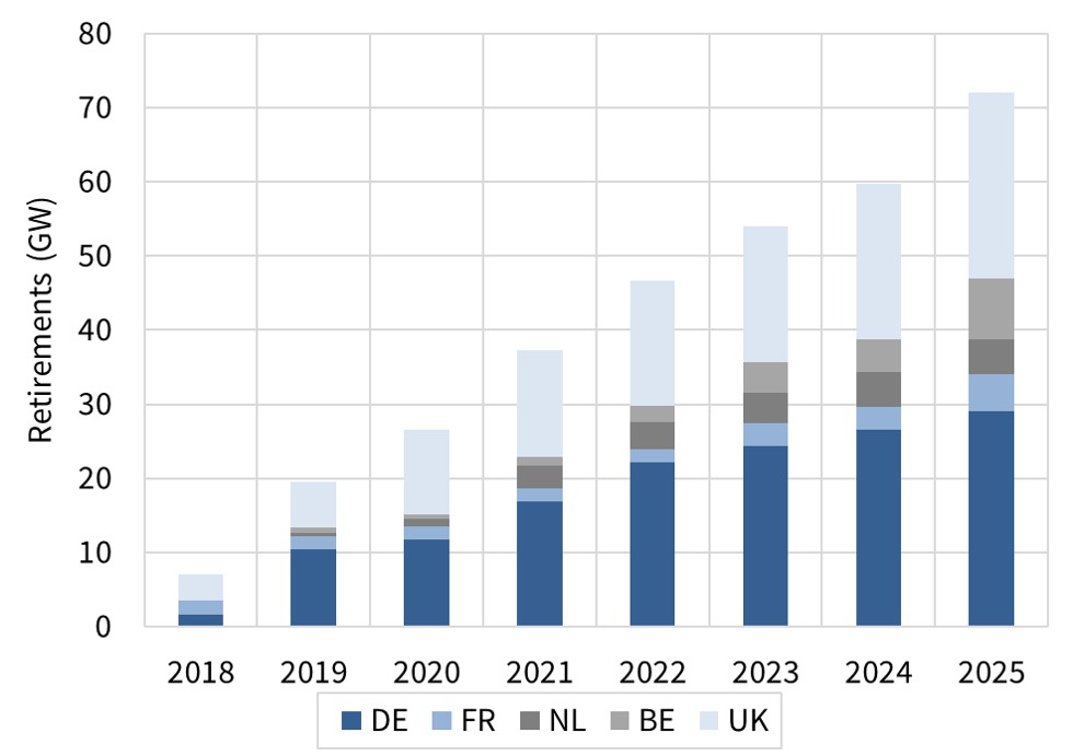
The Mar 30 plan schedules closures of 1GW in 2022, 1GW in 2023 and the remaining 3.9GW in 2025.

These units currently make up 27% of Belgian capacity (5.9GW of a total 22GW), but they account for approximately 50% of Belgium’s generation output.

The easiest solution for replacing lost generation output would be to import more power. But Belgium’s regulatory authorities and system operator have clearly stated they do not want to increase import dependency for security of supply reasons.

So it is clear Belgium needs replacement capacity. What is not clear is where that capacity will come from.

Can renewables plug the gap?

Belgium currently has approximately 3GW of wind and 3.5GW of solar capacity. Based on current policy support mechanisms, technology cost reduction curves and recent build rates, it is our view that Belgium can develop an additional:

~3GW of wind by 2025 (dominated by offshore)
~2GW solar by 2025.

In addition, we assume development of ~1GW of gas peaker capacity (dominated by distribution connected reciprocating engines) and ~0.5GW of battery storage by 2025.

This results in the nominal capacity mix scenario shown in Chart 1 (which also accounts for end of life retirements of some older thermal capacity). This scenario assumes no new large-scale gas build, consistent with a current lack of policy & market price signal support.

Chart 1: Scenario for evolution of Belgium capacity mix – assuming no large-scale gas build

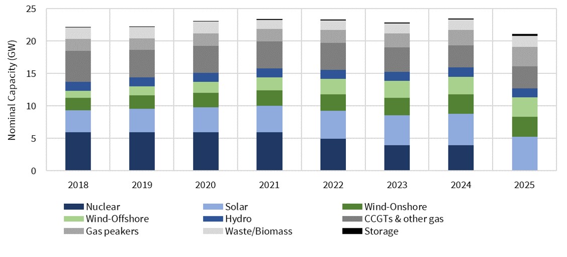
Chart 1 however does not reflect the true security of supply problem Belgium faces replacing nuclear with wind and solar capacity. Wind and solar output needs to be derated to reflect the equivalent firm capacity that can be relied on given load factor fluctuations.

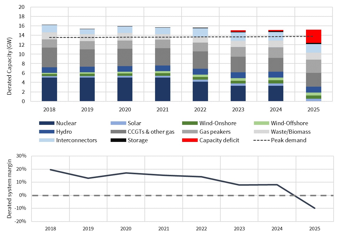
Once 3GW of wind and 2GW of solar build is derated, it yields only about 1GW of equivalent firm capacity. This leaves an almost 3GW capacity deficit in the Belgian market by 2025, with the derated system reserve margin plunging into negative territory as illustrated in Chart 2.

Chart 2: De-rated Belgium capacity mix

What if our renewable build assumptions in the scenario above are too conservative? Even with much more aggressive policy support, it is difficult for Belgium to develop more than 1.5GW of equivalent firm renewable capacity by 2025. This would still leave a ~2.5GW capacity deficit to be filled.

Where is the price signal for flexible capacity?

A 3GW capacity deficit is not a massive technical challenge. Two large CCGT plants would plug the gap. But this solution may be inconsistent with the backdrop of decarbonisation.

Firstly from a policy standpoint, Belgium is likely to be wary of large scale new gas build from an emissions reduction perspective.

Secondly from an economic standpoint, it will be hard to find investment capital willing to commit to new CCGT projects (with 20 year economic lives) commissioning mid next decade. Investors face unpalatable margin risk relying on wholesale price signals alone, as well as the broader risk of stranded assets (as Dutch coal plant developers are painfully discovering).

If Belgium is going to plug its capacity gap with new gas plants, a clear price signal will be needed to secure investment. Belgium has no plans to implement a capacity market (as have the UK, France and Italy). Instead it gained EU state aid approval in Q1 2018 for a strategic reserve mechanism.

Belgium’s strategic reserve initially covers 5 winters from 2017-18. Reserve capacity sits outside the energy market and is called on only in periods of security of supply emergency. As such it can be used to prevent uneconomic older plants from closing. But it is unlikely to send a clear capacity price signal to support new build of flexible capacity.

CHPs may play a role in plugging the 3GW capacity deficit. This could either be smaller distribution connected CHPs (easier but lower volume) or large-scale grid connected assets (more challenging). But adequate policy support mechanisms to deliver significant volumes of CHP are not yet in place.

Where does this lead?

If nuclear plants are closed by 2025, it is difficult to see how Belgium can maintain (i) security of supply and (ii) similar levels of wholesale prices without 2-4GW of new gas-fired capacity. But it is not clear how this capacity will get built in the absence of new policy measures.

The capacity gap may be reduced somewhat by a combination of aggressive role out of renewables & storage as well as tolerance for higher import dependency. But these measures are unlikely to be enough.

There is recent evidence from 2014-15 of the impact of a rapid reduction in Belgium nuclear capacity. Prices separate from neighbouring markets and volatility jumps, with a focus in winters, peaks and periods of lower renewable output. Higher Belgium prices can also drag up French and Dutch prices as imports increase.

Belgian policy makers may be forced to confront the reality that the current path they are proceeding down is not going to work. But they are in good company.

Their biggest neighbour Germany is facing a similar, but much larger problem as it tries to close nuclear, coal and lignite capacity in parallel. We’ll come back soon to address the German problem and its implications for other European power markets.

Timera is recruiting power analysts
We are looking for a Senior Power Analyst and a Power Analyst with strong industry experience. Very competitive & flexible packages. Further details at Working with Timera.

Power sector switching is driving gas hub prices

Posted on May 21, 2018January 16, 2020 by David Duncan

“Everything comes back to gas prices”.

It is not only direct participants in the European gas market that are concerned about the path of hub prices. The direction of TTF and its satellite hubs has a much broader impact across energy markets. For example:

Thermal power: Power assets exposed to wholesale power prices have a strong indirect exposure to gas prices. This is the result of the important influence of hub prices in setting power prices across Europe (which is increasing as coal & nuclear plants close).
Renewables: Gas price influence on wholesale power prices also drives the relative competitiveness of renewables versus alternative capacity types (particularly important for the transition to standalone renewable investment).
LNG market: Europe’s role as swing provider to the LNG market means that European hubs underpin global LNG spot prices, with regional markets pricing off a basis to TTF.

In an article two weeks ago we set out the current state of supply and demand balance in the European gas market. Today we analyse in more detail the drivers of hub price evolution over the next few years with a particular focus on the importance of gas vs coal switching in the power sector.

Unusual uncertainty over next 3 years

The growing importance of gas prices for asset value sits against a backdrop of rising uncertainty as to hub price levels.

In our view, the distribution of potential hub price evolution across the next 3 years is an unusual shape. Rather than a classic ‘bell curve’ normal distribution, there appears to be an unusually broad and flat distribution of potential outcomes.

We also believe this distribution is asymmetrically skewed to the downside as the result of an oversupply of LNG over the next 3 years. In other words, the risk of lower prices is greater than that of higher prices.

Current TTF forward gas price levels are around the 6.5-7.5 $/mmbtu range across 2019-21 (18.8-21.7 €/MWh). To illustrate gas price uncertainty, it is relatively easy to define credible scenarios that deviate significantly from these price levels, e.g.

Price slump: where hub prices fall 40% by 2020-21 to around 4.0 $/mmbtu (11.6 €/MWh) e.g. if European LNG imports rise sharply and coal prices decline.
Price rise: where hub prices rise by 20%+ into the early 2020s e.g. if coal prices rise strongly and Asia comfortably absorbs new LNG supply coming to market.

Switching of gas for coal plants in the power sector is a key mechanism driving marginal hub price levels within this distribution.

Switching as a driver of gas prices

Switching is a relatively simple concept. As gas hub prices fall, gas-fired power plants become more competitive relative to coal plants, with load factors and gas burn increasing accordingly.

This creates additional gas demand and supports hub prices. The process works in reverse as hub prices rise.

This switching mechanism happens in real time based on spot gas, coal and carbon prices. It also influences relative movements in forward gas prices (based on future switching impact).

In order to analyse the role of switching in driving European hub price levels, it is useful to apply a three step framework:

LNG surplus: determine what volume of surplus LNG may flow into European hubs over the next 3 years
Switching: define how volumes of surplus LNG can be absorbed by power sector switching and at what combination of gas, coal (& carbon) prices
Gas price impact: determine the hub price levels required to balance the European gas market (& therefore the global LNG market given Europe’s role as swing provider)

We looked at the volume range of potential LNG surplus (1.) in last week’s article. In today’s article we put some numbers around 2. and 3. (switching potential & hub price impact).

Defining the switching range

Chart 1 illustrates the hub price range over which switching is important (shaded in blue). It shows this in the context of the current differential between TTF forward prices and US Henry Hub. Backwardation in the current forward curve can be seen in the relative price decline from 2019 to 2021.

Chart 1 Gas hub prices and the switching range

Source: Timera Energy

The top end of the switching range is defined by the point at which the UK power sector (with its carbon price floor) switches all its coal capacity back into merit (significantly above 8.0 $/mmbtu).

The lower end of the switching range is defined by the point at which US LNG export ‘shut ins’ transition to be the primary mechanism for absorbing surplus gas. Shut ins occur if the variable costs of exporting US LNG falls below netback spot prices. This is likely to happen if European hub prices fall below a 0.7-1.5 $/mmbtu variable LNG transport cost differential to Henry Hub (marked as the grey shaded area).

Switching continues in the grey ‘shut in’ range. It is just that shut ins are a much more dominant volume driver once gas prices fall to this level, given the ability for relatively large volumes of US export supply (80+ bcma) to be shut in over a relatively narrow price range.

Switching demand curves

It is one thing to understand the range over which switching is a dominant driver. It is another to define switching price & volume levels and their impact on hub prices.

In order to perform a robust analysis of aggregate gas vs coal switching potential in Europe, it is important to model the underlying dynamics of the individual power markets which drive switching. To enable this, we have set up a scenario in our pan-European power market model that reflects current forward market pricing for fuels. This provides a benchmark for aggregate power sector gas demand given current gas and coal market prices.

We then run multiple combinations of gas and coal prices through the power market model, in order to analyse aggregate pan-European gas vs coal switching potential. This allows us to produce gas switching demand curves for the different combinations of gas & coal prices shown in Chart 2.

Chart 2: Pan-European switching demand curves

Source: Timera Energy

Each line in the chart can be thought of as an aggregate gas demand curve for the European power sector. In other words, the lines show aggregate gas burn (bcma) as a function of gas price. Three different demand curves are shown for different coal prices.

The central line shows switching dynamics at current forward coal prices for European delivery (approximately 90 $/t). As you move from left to right down this line, gas switching volume increases as gas prices fall.

For example, a fall in gas prices from the 2019 forward price level (7.3 $/mmbtu, 21.2 €/MWh) to the ‘shut in’ range (4.2 $/mmbtu, 12.2 €/MWh) yields about 30 bcma of incremental switching demand, assuming coal (& carbon) prices are constant.

Coal prices typically move with gas prices (although not always in a correlated way). In order to understand the impact of changes in coal prices, we have also produced switching demand curves for coal prices 30 $/t above and below the 90 $/t central case (at 60 and 120 $/t).

As an example, if coal prices were to rise to 120 $/t, European hubs could support similar levels of power sector gas burn at prices around 1.7 $/mmbtu (4.9 €/MWh ) above current levels. This example illustrates why hub prices are currently rising with coal prices as switching levels increase accordingly.

Conclusions on gas price levels

In last week’s article we set out the potential volume range of LNG that may be surplus to ‘business as usual’ requirements in Asia & Latin America (15-70 bcma in 2020). Not all of that surplus LNG will flow to Europe.

There is likely to be some incremental demand response in Asian markets at lower spot prices (e.g. 10-20 bcma of additional demand if prices fall below 5.0 $/mmbtu). But there is certainly a credible risk in our view that 40+ bcma of surplus LNG could flow to Europe by 2020-21 in a scenario of weaker Asian demand growth.

Our switching analysis shows 20-30 bcma of accessible incremental switching potential in Europe, before hub prices fall to US shut in levels. This switching volume would rise if coal and/or carbon prices continue to increase.

If surplus LNG flows to Europe remain below this 20-30 bcma level, then switching should allow hubs to absorb extra cargoes (e.g. in a 5-7 $/mmbtu price range based on current coal/carbon prices).

But if surplus LNG imports into Europe rise above 40 bcma, it is hard to construct a scenario where US shut ins are not required. That would likely mean European hub prices at levels below 4.5 $/mmbtu (13.0 €/MWh), maybe as low as 3.5 $/mmbtu (10.1 €/MWh).

We are not predicting this low price scenario, but it is a credible downside risk flashing on the radar screen. And it represents a substantial deviation from current forward price levels.

LNG oversupply setting up 2020s squeeze

Posted on May 14, 2018January 16, 2020 by David Duncan

‘There is an LNG glut’. ‘No, the market is tight’. Two tribes have emerged within the LNG market and their views are polar.

The glut tribe argues that LNG supply will outpace demand growth over 2018-21, forcing spot prices lower, potentially towards 4 $/mmbtu in order to shut in US exports.

The tight market tribe sees little evidence of oversupply, given demand growth is broadly keeping pace with new liquefaction projects coming online. It also points to a shortage of gas in the early 2020s due to a lack of investment now.

The key element that is often missing within this polarised debate is timing. If appropriate time horizons are defined, it is quite possible both tribes will be proven right. In fact oversupply over the next three years may be a powerful catalyst for a tightening market in the early-mid 2020s, as it chokes off liquefaction investment decisions.

New investment has dried up

Significant uncertainty around the level of Asian LNG demand has fueled the polarisation of industry views. It is generally accepted that cargoes which are surplus to Asian & Latin American requirements will flow to Europe. But the level of this surplus could quite credibly be anywhere from 15 – 70 bcma (10-50 mtpa).

Chart 1 shows the global LNG market balance under an illustrative high and a low Asian demand scenario. The global surplus of LNG (vs business as usual demand) is shown by the hashed red area above the balance line. Beyond this, the global deficit of LNG is shown by the red shaded area below the line. The period in between surplus and deficit reflects the ability of Russian pipeline exports to temporarily meet incremental demand growth requirements with shut in West Siberian gas production.

The scenarios in Chart 1 illustrate both the time & volume range of global surplus LNG volumes that could flow to Europe depending on Asian demand growth:

The top panel shows a more aggressive Asian demand scenario with only 16 bcma surplus flow in 2020 and new supply required by 2022
The bottom panel shows a slower Asian demand scenario with 61 bcma of LNG surplus in 2020 and a requirement for new supply from 2024.

Chart 1: Illustrative range of surplus LNG flows into Europe depending on Asian demand

Source: Timera Energy

Volumes towards the lower end of this surplus range can be absorbed at European hubs in a relatively orderly fashion via power sector switching. Volumes at the upper end of the range are likely to force European hubs down from current levels (~ 7 $/mmbtu) to levels that shut in US export flows (~ 4.0-4.5 $/mmbtu assuming Henry Hub prices remain ~ 3.0 $/mmbtu).

This uncertainty is causing Financial Investment Decisions (FIDs) in new liquefaction capacity to dry up. There was only one liquefaction FID in 2017 – ENI’s Coral South FLNG project.

The next wave of investment looks to be some way off

Market uncertainty also means there are few credible prospects for FID in 2018. The winter surge in Asian spot prices supported some optimism in late 2017. But this was largely the result of a lack of seasonal storage in Asia, with prices quickly re-converging with European hubs in Q1 2018.

Cheniere is expected to make a decision this year on Corpus Christi Train 3 (cost advantage given existing infrastructure). Ophir’s Fortuna FLNG project FID was expected this quarter but appears to have been delayed by issues with financing. It is slim pickings for imminent FIDs beyond these projects.

Liquefaction projects typically have a 4 to 5 year lead time to full production. That means FIDs taken in 2018 are unlikely to impact global supply until 2022-23. Glut or no glut, the pace of new supply entering the market is set to accelerate over the 2019-20 period. This will likely keep a cap on LNG prices and new project FIDs.

So it may not be until the early 2020s that significant volumes of new investment are forthcoming. That is likely to be too late. The timing of Qatar’s decision to bring 20+ mtpa of low cost new supply to market will be key. But as things look today, the LNG market may be marching towards a major squeeze in the early-mid 2020s.

Winners & losers from an LNG price surge

The key losers from higher gas prices are consumers (residential, commercial and industrial). Retailers may also be hurt, to the extent they cannot pass through price rises e.g. for contractual, competitive or policy reasons. Gas-fired power plants would also likely suffer from an erosion of competitiveness versus coal plants.

A gas price surge would clearly benefit gas producers (although this is dependent on timing & offtake contract structures). A tighter market would also likely mean greater gas price volatility, paying dividends to owners of flexible midstream assets e.g. LNG portfolio players.

There would also be important knock-on impacts for European power markets. By the early 2020s, gas-fired plants will dominate marginal setting of wholesale power prices. That means higher gas prices translate directly into higher power prices (via CCGT pass through). That is good news for the prospects of standalone renewable development. But it may also prolong the economic lives of coal plants (depending on coal & carbon prices).

European gas balance: drivers & prognosis

Posted on May 7, 2018January 16, 2020 by David Duncan

European gas demand hit its ‘high-water’ level of 586 bcm in 2010. From 2010 to 2014 demand then reversed sharply, falling 19% (111 bcm), and commencing what many perceived to be an irreversible downward trend.

This trend was generally accepted to be in line with the growth of renewables in the power sector (at the expense of gas) and the slow demise of energy intensive industries in Europe as these were ‘offshored’ to developing Asia.

This script conveniently aligned with EU policy. It was consistent with reduced reliance on Russia as the largest source of natural gas imports. This was important given several points of disagreement between the EU and Russia. For example, territorial infringement in Ukraine, the issue of Nordstream 2 versus maintenance of transit flows (and revenues) through Ukraine, and squabbles over the use of downstream pipeline capacity related to Nordstream 1.

If reduced natural gas consumption was the EU policy ‘game plan’, the reality from 2016 onwards makes for uncomfortable reading. European gas demand has rebounded almost as quickly as it fell. And overwhelmingly, Russia has been the supplier benefitting from this.

What is driving demand growth

European gas demand has recovered 16% (77bcm) across 2014-17. This rebound has been surprisingly consistent across countries: UK 4.1%, Germany 6.0%, Italy 6.7%, France 5.5%, Netherlands 4.9%, Spain 4.8%, Turkey 3.2%, Belgium 4.3%, Others 5.5%.

A recovery in economic & manufacturing growth has played an important role, particularly in 2016-17. Lower wholesale gas prices since 2014 (relative to earlier in the decade) have also helped support demand. But Chart 1 illustrates that one of the pillars of gas demand recovery has been power sector consumption.

Chart 1: Power sector gas demand across 5 largest markets

Source: Timera Energy

Gas demand from power generators across these five markets accounts for ~30 bcma of the gas demand rebound since 2014. This is partly the result of gas for coal switching that has taken place given:

Coal prices strengthening relative to gas prices
A step up in the UK carbon price floor (to 18 £/t in Apr 2015)

However there are also some ‘one-off’ factors that have supported power sector demand e.g. the French nuclear outages in Winter 16/17 and low Spanish hydro availability in 2017.

The extent of power sector gas for coal switching over the next 3 years will be a key factor determining whether European gas demand continues to recover or stalls.

Where is new supply coming from?

Chart 2 shows the dominance of Russia in meeting demand growth since 2014, with Russia providing 45bcm of the 77 bcm European growth.

Chart 2: Evolution of key sources of European gas supply (2010-17)

Source: Timera Energy

Domestic European production has been in general decline since 2010, although this decline has stabilised somewhat over the last two years. This is partly due to strong Norwegian flows. But some UK production, which achieved FID during the high oil/gas price conditions of 2011–14, has also come onstream.

Non-Russian pipeline imports have been variable. It is thought that Algeria’s 2016 increase was achieved by ‘borrowing’ Hassi R’Mel recycle gas in advance of new fields coming onstream. Apart from the anticipated boost from Azerbaijan’s Shah Deniz 2 around the end of this decade – there is little prospect of an increase in non-Russian European pipeline gas imports.

LNG imports were around 90 bcma in 2010 and 2011, when new LNG supply projects hoping to target the US ended up in Europe by default (as a consequence of the US shale gas revolution). As Asian LNG demand has grown since then, it has drawn LNG away from Europe. 2017 saw a break in this trend. Growing global LNG supply caused European imports to increase by 20% over 2016 levels, though this was mainly confined to Southern Europe.

Higher LNG imports are the only substantial threat to Russia dominating incremental supply volumes into Europe. Surplus LNG cargoes flow into Europe as ‘price taking’ gas (i.e. insensitive to price while prices remain above US export shut in levels). But so far the volumes of surplus LNG imports into Europe have been well below demand growth, allowing Russia to step into the gap.

What next?

Some of the factors behind the rebound in European gas demand are unlikely to support further consistent demand growth. For example:

UK has limited additional coal switch-out potential
French nuclear capacity has returned to higher availability (at least for now)
Drought/hydro issues revert to mean (which may be negative for gas demand)

But there are 5 structural drivers of the European gas market supply & demand balance we are keeping a close eye for guidance on what may happen next:

Switching: Relative coal vs gas prices and associated power sector switching volumes
Capacity mix: Pace of retirement of (i) coal, lignite & nuclear capacity & (ii) growth in renewables capacity
Economic growth: Extent to which non-power sector gas demand continues to rise
Domestic production: Pace of production decline (e.g. across Groningen, UKCS)
LNG imports: Volume of surplus ‘price taking’ LNG flow into Europe

We will return to look at some of these drivers in more detail as the year progresses.

At the flicks: gas curve animation

Posted on April 30, 2018January 16, 2020 by David Duncan

Energy markets are awash with charts. We work in a data intensive industry and a good chart can be worth a thousand words. But charts by nature provide a static view of factors such as price, volume, value & risk.

Chart animation adds an additional dimension: time. That can help a lot with interpreting the dynamic evolution of market prices and let’s face it, everyone likes a trip to the movies.

Today we animate the evolution of NBP gas prices. We’re no threat to Pixar, but the animation supports some interesting takeaways on current gas pricing dynamics.

The NBP snake

Chart 1 shows the simultaneous evolution of NBP spot and forward gas prices. The strong arbitrage driven relationship between NBP and TTF means that many of the characteristics of this animation apply for TTF also. But we’ve chosen NBP rather than TTF to focus on some recent pricing dynamics that are specific to the UK.

Chart 1: NBP gas curve animation (2010-18)

Source: Timera Energy (based on ICE data)

Some takeaways to consider

1. Spot vs forward: there is a very strong relationship between spot prices (we’ve used month-ahead prices in Chart 1) and shifts in the forward curve (‘spot wagging the curve’), although this can break down in periods of more extreme spot price stress.
2. Winter 17/18: NBP month-ahead prices took off in Dec 17 due to a combination of supply outages and uplift from high spot LNG prices given strong Chinese demand for spot cargoes. However the ‘beast from the east’ day-ahead and within-day spikes in Feb 18 had very little impact on forward prices (given short term weather driven nature of the shock).
3. Seasonal spreads: UK seasonal spreads can be seen roughly doubling from 2016-18 (4 to 8 p/th) to induce more supply flex since the closure of Rough. Front year spreads can be very volatile as spot prices move.
4. Recent spot price ramp: European near term gas prices are again being pulled higher by rising coal prices in Q2 2018. Higher coal prices lifts gas for coal plant switching levels in the power sector which provides support for gas prices.
5. Current backwardation: European gas curves (like the Brent crude curve) are also moving into strong backwardation which is relatively unusual for gas. This is due to a combination of (i) rising spot prices and (ii) the looming ramp up in surplus LNG acting to dampen forward prices across 2019-21.

The other important thing to note is that current NBP/TTF forward curves are consistent with Europe comfortably digesting surplus LNG this decade (at annual prices above 6 $/mmbtu). European hub spreads vs US Henry Hub (3-3.50 $/mmbtu) are well above the variable costs of flowing US exports to Europe. The Q1 2016 price slump has so far been the only time when the trans-Atlantic spread declined to levels that threaten US shut ins.

We will be back soon to revisit how Europe can digest surplus LNG via gas vs coal switching and the associated impact on hub pricing dynamics.

Plant closure: Valuing closure option vs alternatives

Posted on April 23, 2018January 16, 2020 by David Duncan

Plant closure decisions are usually driven by expected profit. But a simple assessment of plant profitability is usually an inadequate approach to inform a plant closure decision.

This needs to be couched within a structured investment decision framework that maps out:

Alternative options (e.g. cost restructuring, refurb, conversion, mothball, repower, reserve contracts)
Timing of exercise (often driven by external factors e.g. technical, policy or market related)
Cost of exercise & in some case cost of carrying options
Risk adjusted value of exercise (using a probabilistic approach)

A robust investment decision framework allows a plant owner to quantify and assess the risk/return distributions of alternative options as the plant progresses towards closure.

Today we follow on from last week’s article on drivers of plant closure by exploring a practical case study of CCGT end of life investment decisions.

CCGT closure vs life extension

CCGT plants usually face a key investment decision around 25 years of age. The exact timing depends on technology, run hours and operation profiles. But life extension beyond this point typically requires major capex spend e.g. relating to replacement of steam generator components.

This life renewal capex hurdle may trigger plant closure if analysed in isolation, but there are usually several other options available to plant owners, for example:

GT conversion: Bypassing the steam generator to run the gas turbines alone (lower efficiency but often with associated fixed cost reductions)
Refurb: capex spend to extend plant life and increase flexibility e.g. reducing minimum stable generation levels and start costs to enable greater capture of prompt, balancing & ancillary revenues
Repower: Replacement of existing generators with new equipment, but re-using site infrastructure
Mothball: Substantially reducing fixed costs to retain the option of reopening the plant in the future (this only makes sense for certain assets and market conditions e.g. Netherlands and Germany both have significant mothballed CCGT capacity in anticipation of a tightening capacity balance).

A structured approach is required to properly quantify and compare the relative risk/return of these different options. This requires a robust probabilistic plant modelling framework that generates realistic distributions of asset margin under each of the alternative options.

A nodal decision tree can then be constructed to estimate risk adjusted values for different investment options as illustrated in Chart 1.

Chart 1: CCGT closure vs life extension option decision tree

Source: Timera Energy

This framework can be assessed for example on an annual basis as the plant ages and market & operational conditions change. But it is important to note that options are impacted by decisions taken i.e. there is a ‘path dependence’ problem that needs to be properly analysed and accounted for.

DCF / NPV calculations to support investment decisions may require use of multiple discount rates, depending on the nature of the uncertainties associated with the various options (which can be very different).

Mid-life asset ownership is becoming a specialist game

It is no coincidence that commodity traders and private equity firms are buying mid-life thermal power assets across Europe (e.g. KKR French CCGTs, Vitol Immingham CCGT, Castleton Rotterdam CCGT, ECP Saltend & Deeside CCGTs).

The changing ownership of thermal assets reflects:

More challenging risk/return profiles of assets as they age, load factors decline and value becomes more focused in the prompt horizon
More complex investment optionality as assets enter later life (as per case study above)

The first of these factors requires a strong trading capability (either in-house or via route to market contract). The second factor requires strong expertise on plant investment optionality & cost structuring.

Applying the investment approach we describe above can unlock significant upside value from ageing assets. This is a key factor behind the increasing trend in change of ownership of mid-life thermal assets, as traditional utility owners sell to specialist investors.

Plant closure: drivers of the decision to close

Posted on April 16, 2018January 16, 2020 by David Duncan

European power markets are facing a demographic issue. Flexible thermal generation capacity is ageing at a faster rate than it is being replaced.

This phenomenon is consistent with the intentions of policy makers as Europe moves towards decarbonization of the power sector. Thermal capacity is steadily being replaced by investment in renewable generation assets.

But new capacity is strongly skewed towards low variable cost and relatively inflexible wind & solar generation. This means the flexibility of remaining thermal power plants is playing an increasingly important role in ensuring power system security of supply.

Low carbon sources of flexibility such as load shifting storage & demand side response are evolving quickly. But evolution of technologies, cost curves and policy support for these low carbon flex sources means that even under optimistic scenarios, Europe will rely on thermal generation flexibility well into the 2030s.

This means that European power markets face a balancing act over the next decade as they progress towards decarbonization. Part of this equation is about investment in new flexible capacity including new low carbon technologies. But capacity demographics are as much about plant deaths as about plant births.

In this context, we focus our next two articles on plant closures. Today we look at economic and other drivers of owners’ decisions to close plants. Then next week we set out a structured investment framework for assessing plant closure decisions.

Closure is more complex than just profitability

Simple investment logic points to plant closure decisions based on profitability. But it is important that profit is viewed from an economic rather than an accounting perspective. By this we mean making decisions based on opportunity costs.

All sunk costs should be excluded from the decision to close a plant. Closure economics should be based on an evaluation of avoidable costs. This is often not straightforward. For example in the context of a UK capacity auction cycle, more costs are avoidable four years ahead of delivery (T-4) compared to one-year ahead (T-1).

All other things being equal, these avoidable costs need to be covered by an adequate level of risk-adjusted revenue, to justify keeping the plant open. Although this concept seems simple, there is usually a complex interaction across a number of value drivers behind it. We summarise these in Table 1.

Table 1: Value drivers of plant closure

Driver	Description	Considerations
Margin uncertainty	Uncertain evolution of wholesale, capacity & balancing/ancillary margins	Large impact on closure economics Probabilistic quantification required Margins need robust risk adjustment Some risks can be hedged Risks increase as load factors decline
Sunk costs	Defining which costs are truly avoidable by closing plant	Important to define over what timescales closure costs become sunk or triggered e.g. rates, insurance, operations & maintenance, redundancy
Cost uncertainty	Elements of cost evolution can carry uncertainty	Many elements of plant cost are stable But some assets face significant uncertainty e.g. potential IED policy costs; transmission charge evolution
Cost reductions	May be options to reduce some plant costs	Assessing options for reducing plant costs can extend asset lives For example, changing station operational patterns & staffing structures; renegotiating O&M contracts
Decomissioning costs	Timing of incurring decommissioning costs can be a significant economic driver	NPV impact of decommissioning cost timing can be substantial, particularly for coal plants
Alternative options	Closure economics need to be consistently assessed against alternatives	Economics of alternatives also need to be quantified, e.g. refurb, mothball, repower Paying an ‘option fee’ to enhance a plant can generate attractive value upside
Other risks	Performance of ageing assets needs to be appropriately risked	Plant performance (outages, efficiency & flex) typically erodes as a plant ages Dispatch profile can significantly increase outage rates (e.g. higher ramping & starts)

Source: Timera Energy

Closure timing and triggers

The precise timing of a closure decision can often be triggered by major cashflow related events that impact the plant. An example of this in a UK, French or Italian market context is exit from a capacity auction (given associated loss of capacity revenue). Other events that can trigger closure include cashflows related to major overhauls, debt repayments and the need to meet changing environmental legislations (e.g. IED capex decisions on coal & lignite plants in Germany).

There can be important practical implications of decommissioning cost liabilities. For example tax and accounting treatment of balance-sheet decommissioning provisions can influence optimization of closure timing. So can the extent to which decommissioning provisions differ from estimated decommissioning costs. Regulatory risk around decommissioning costs is also a consideration, with decommissioning & clean up obligations typically becoming more onerous over time, typically favouring earlier closure.

Closure decisions can also be impacted by codependence with other units on the same site or in the same portfolio. For example, by closing one unit at a four-unit station it is unlikely that a quarter of fixed costs will be saved. Instead, fixed costs are spread over a smaller base and look more expensive from a CFO’s perspective. This may set the bells ringing for the remaining units.

Why decisions can deviate from plant economics

There may be rational explanations for plant closure decisions to deviate from those implied by a purely economic assessment. A good example of this is the portfolio effects of closure. From a strategic bidding perspective in the UK capacity market, portfolio players mays consider the impact of marginal closure decisions of certain plants on the rest of their portfolio. Portfolio value impacts may be driven by the clearing price on the remainder of portfolio generation assets or on costs passed through to integrated retail businesses.

There may also be behavioural or other factors in play that are not obvious from an external economic assessment e.g.

Self-fulfilling prophecy: as closure looms, owners have a tendency to cancel/defer discretionary maintenance, often pushing the plant down an irrecoverable path to closure
Grasping at straws: working in the opposite direction, owners can clutch for excuses to keep a plant (& associated options) alive, even if economics point to closure
Recent acquisition bias: A recent acquirer of a plant may be anchored to pre-acquisition assumptions on market & margin evolution
Last man standing: ‘If everyone else closes first my plant’s value will recover’, or a blind hope variation ‘something will turn up to save us’
Broader perspective Boards can often be reluctant to make politically sensitive or reputationally sensitive decisions around plant closures
Turkey voting for Christmas: a management team working with a portfolio of one plant may not make the same recommendations as a manager with a portfolio of a dozen units

Whether the drivers of closure decisions are economically rational, behaviorally rational or otherwise, these factors all have an important practical impact on plant closure timing. But that does not mean owners should step away from a structured economic assessment of closure decisions.

Large sums of money can be made or lost in optimizing the options associated with a thermal asset approaching the end of its life. We set out an investment decision framework for the assessment of closure vs alternative options in next week’s article, including a practical case study for CCGT assets.

Russian & LNG imports: a rebalancing act

Posted on April 9, 2018January 16, 2020 by David Duncan

German and Finnish approval of the Nordstream 2 pipeline over the last two weeks helps pave the way for Russia to continue its role as predominant gas exporter to Europe.

Russian gas will compete with LNG supply to meet growing European import demand in the 2020s. But will Russian or LNG imports replace the seasonal flexibility that Europe is losing from maturing domestic production?

Plenty of Russian gas but seasonal profile is declining

Vast reserves in Western Siberia mean there is no imminent prospect of declining Russian gas production. There is an estimated 100bcma+ of shut in Russian production developed as the result of overly optimistic European gas demand forecasts last decade.

Russian exports to Europe have in fact been steadily increasing since 2015. But as flow volumes have increased, the seasonal profile of Russian imports has declined.

In our last article we set out how maturing production was causing a decline in seasonal flex from the UK, Netherlands and Norway. In the case of Russia, loss of seasonal flex is driven by changing flow routes and strategy rather than upstream issues.

Gazprom has made a clear strategic decision to bypass the traditional Ukrainian flow route to the extent that capacity is available on other routes. This strategy is set to continue given:

Significant historical transit losses and ongoing political tensions with Ukraine
Nordstream 2 facilitating additional flow volumes via northern routes into Europe.

As part of this strategy, Russia has also substantially reduced its usage of Ukraine’s vast gas storage assets. This has effectively eroded the provision of flex from Ukrainian storage to the European gas market. The loss of seasonal profile from Russian flows has been reinforced by Gazprom more actively marketing uncontracted volumes at European hubs across the summer months (having overcome its previous aversion to selling at spot prices).

The reduction in the seasonal flow profile of Russian imports can be seen in Chart 1.

Chart 1: Russian flow volumes by key routes to Europe this decade

LNG imports providing the wrong sort of seasonality

As domestic production declines, incremental LNG imports will be the other key source of supply growth into Europe. LNG flows reflect regional supply & demand balances and price spreads. This means LNG provides a very different sort of flex to Russian gas.

The LNG market can deliver Europe large incremental volumes of gas at the right price. But the supply chain for LNG is more complex than for pipeline supply. And it takes longer to respond to market price signals, typically from 2-6 weeks to deliver a material increase in volume.

There are however growing structural trends in the way LNG flows into Europe. An increasing shortage of domestic storage in Asia (particularly in China) is causing flexible LNG cargoes to be diverted away from Europe across the winter. This dynamic has been clear over the last two winters as Chinese LNG demand has surged.

A similar logic tends to cause surplus LNG to flow into European hubs across the summer months. In other words, European LNG imports are increasingly displaying a counter-seasonal profile which is compounding the loss of seasonal shape from domestic production.

Flex market rebalancing

In our last article we set out why Europe faces an unambiguous decline in seasonality from domestic production. The earthquake induced pace of reductions in Groningen production, now targeted to cease production by 2030, is accelerating this dynamic.

In today’s article we have explained why structural trends driving Russian and LNG import profiles are also reducing the seasonal shape of flows into Europe.

For the last decade the European gas market has experienced an oversupply of seasonal gas flexibility. This was the result of weaker than expected gas demand, overbuild of storage and improved optimisation of existing portfolio flexibility.

However investment in seasonal flexibility has dried up at the same time structural trends are eroding existing seasonal flex. Over the last five years, seasonal price spreads at European hubs have been crushed towards the variable cost of cycling seasonal storage assets (1.0-1.5 €/MWh). It may be complacent to assume that spreads remain at this level for the next five years.

European production flex is declining fast

Posted on March 26, 2018January 16, 2020 by David Duncan

Europe faces a structural decline in domestic gas production. Domestic output (excluding Russia) is set to decline from 252 bcma in 2017 to 150 bcma by 2030.

This trend of declining production is well understood. But the associated decline in supply flexibility and seasonality of production flows is less so. Rapid declines in Groningen output and maturing Norwegian production are combining to erode domestic supply flexibility in Europe.

In this week’s article we consider the scale of lost domestic production flexibility. Then in our next article we look at how changes in Russian export strategy and flow routes are also impacting supply flexibility.

Breakdown of key domestic supply sources

Three main sources of domestic production have historically provided substantial seasonal flexibility to the European gas market. But maturing production, ageing assets and falling upstream capex investment are reducing both the level and seasonality of flows.

Netherlands

Earthquake related production cuts have reduced Dutch gas production by 70% since 2013. This year’s latest 12bcma cap has also substantially eroded Groningen’s seasonal production profile.

Prior to 2013, the Netherlands historically provided a seasonal swing of 6-7 bcm of monthly output from highest winter month to lowest summer month as illustrated in the top panel of Chart 1. That will fall to less than 1 bcm swing under the new cap.

Chart 1: Historical & projected monthly Dutch gas production (2010-30)

Norway

Norwegian production has plateaued and is set to steadily decline next decade. Norway provides 3-4 bcm peak winter to trough summer month swing. This is likely to fall to under 2bcm later next decade as can be seen in Chart 2.

Chart 2: Historical & projected monthly Norwegian gas production (2010-30)

Norwegian seasonal flexibility has played a key role in ‘backfilling’ the loss of Rough storage in the UK. That has reduced seasonal profile of flows to the Continent.

As well as seasonal flex, Norway provides important daily deliverability flexibility, particularly into the UK gas market. Recent declines in Norwegian upstream capex spend rates are set to impact provison of flexibility over the next 5 years. Reduced performance from the large Troll field could significantly curtail Norway’s supply flexibility in the 2020s.

UK (& other)

The UK has historically been Europe’s third key domestic producer. However UK production declines over the last 15 years have already substantially reduced supply flexibility. The UK peak to trough monthly swing is less than 1 bcm and will decline further with production next decade.

This pattern is also true across other European domestic production (e.g. in Germany, Italy, Poland & Romania) which has a relatively flat profile.

The upshot of declining domestic supply flex is that Europe is rapidly becoming more dependent on imported flexibility. That leads us to look at Russian supply flexibility in or next article. But we will be taking a one week break over Easter first.

NW Europe’s flexible capacity crunch

Posted on March 19, 2018January 16, 2020 by David Duncan

The luxury of oversupply

There has been a structural oversupply of capacity in North West European power markets this decade (with the notable exception of the UK). Excess capacity has been the result of slower than expected demand growth. This has been exacerbated by an overbuild of thermal assets, particularly new coal and CCGT plants in Germany and the Netherlands.

Strong policy support for renewable generation has seen wind, solar and biomass capacity delivered into power markets which already have excess thermal capacity and adequate flexibility to absorb intermittency. Structurally oversupplied markets have shaped policy decisions and investor attitudes to deploying capital.

Retirements pipeline changes the landscape

The NW European power market balance is set to substantially change across the next 5-7 year due to:

Regulatory driven nuclear closures, for example:
1. 10GW in DE by 2022
2. 6GW in BE by 2025
IED & national policy driven closures of coal units, for example:
1. 12GW in UK by 2025
2. ~10GW in DE by 2025 (IED dependent)
3. 3GW in FR by 2022
4. 5GW in NL by 2030
Ageing gas plants will need major lifetime renewal capex or close by 2025, for example:
1. ~10 GW in Germany
2. ~9 GW in UK

Cumulative projected thermal capacity retirements by country are shown in Chart 1, based on currently announced policy measures.

Chart 1: Projected NW European thermal capacity retirements

Source: Timera Energy

These closures will significantly tighten the NW European capacity balance as well as removing substantial volumes of dispatchable flexible capacity.

Policy makers are not blind to this challenge. In February the EU approved a further 6 capacity payment mechanisms (DE, BE, IT, FR, PL & GR). But despite new policy measures there is not yet a compelling investment case to support delivery of new flexible capacity (UK aside).

The requirement for new capacity is clear from a security of supply perspective. But the price signals that will support capacity investment are less clear.

A capacity mechanism tour of NW Europe

UK:

Necessity is the mother of intervention. The UK power market tightened over the first half of this decade as thermal capacity retired. As a result the UK implemented a capacity market that has delivered significant volumes of new flexible capacity.

Capacity investment has been underpinned by 4 year ahead auctions of up to 15 year capacity agreements for new builds i.e. a clear capacity price signal that supports commitment of capital. This approach has not been replicated in other NW European markets.

France:

French security of supply is underpinned by its 63GW nuclear fleet. Despite political rhetoric, there is unlikely to be substantial net closures of French nuclear capacity before 2030. Nuclear is complimented by significant hydro flex and high levels of interconnection. Flexible capacity retirement volumes are likely to be relatively low over the next decade and will predominantly be replaced by a ramp up in renewable capacity.

The French implemented a supplier obligation based capacity market in 2017, with annual capacity payments. In practice this mechanism is likely to be more focused on retaining existing capacity than supporting structural investment in new flexibility. However the French government have provided specific support for new thermal capacity (a CCGT project to alleviate constraints in Brittany) and the newly approved French demand response mechanism may flush out some DSR flex.

Belgium:

Belgium is a step closer to the UK in terms of market tightness. But it is a relatively small market which is very well interconnected (6GW of links with FR & NL). Belgium’s major issue is replacement of 6GW of ageing nuclear capacity between 2022-25. The government and TSO are aiming to do this without a step change in dependency on imported power.

The EU state aid commission approved a Belgian strategic reserve mechanism in Feb 2018. This is focused on an emergency reserve to retain ageing thermal units (that would otherwise close). It may also help some smaller distributed capacity, but it is unlikely to structurally solve the nuclear replacement issue. That suggests that wholesale prices and volatility are set to rise.

Netherlands:

Thermal capacity overbuild has been most acute in the Netherlands. The first half of this decade saw an almost masochistic competitive battle between utilities and independent developers to deliver new capacity volume at the expense of margins. This wounded thermal plant owners, but excess capacity has dampened security of supply concerns for the Dutch government.

The Netherlands has a relatively young and flexible thermal fleet dominated by CCGTs. Ongoing proactive support for renewables is set to fill most of the capacity gap from retiring plants. This means that intermittency will play a more important role in the Dutch supply stack going forward. But capacity developers will need to look to the wholesale market for investment price signals.

Germany faces the biggest capacity challenge

Germany anchors the network of NW European power markets. German thermal capacity dominates regional price setting. Swings in renewable output are also increasingly drawing on regional flexibility, as Germany moves towards its target of a 65% renewable energy share by 2030. The challenge Germany faces is being exacerbated by substantial closures of thermal capacity.

After the Fukushima disaster, Germany decided to close its remaining 12GW of nuclear capacity. We are sceptical of the closure logic from an emissions perspective. But the German government is effectively implementing the plan, with 9.4GW of remaining capacity to close by 2022.

Germany is also likely to close an estimated 10GW of coal and lignite units by 2025. This includes 2.7GW of lignite units currently ring-fenced in a climate reserve. It also covers a number of older coal units that breach IED NOx limits. IED driven closures of coal & lignite may rise to 20GW by 2030, although volume uncertainty remains given potential capex spend to mitigate emissions on some units.

Germany also has an ageing gas plant fleet. CCGTs typically require major lifetime renewal capex to avoid closure at around the 25 year mark (although exact timing is dependent on run hours, technology configuration and operational patterns). Another 10GW of gas-fired units will reach this point by mid next decade, likely resulting in substantial gas plant closures.

Given the scale of thermal closures, Germany faces a structurally different problem to other markets such as France and the Netherlands. German capacity maths does not add up without substantial investment in new flexible capacity. The strategic reserve mechanism that has just been approved by the EU does not appear to solve this problem.

Implementation of the strategic reserve is planned for 2019. The reserve allows payments to existing thermal units that would otherwise close, but support is capped at 2GW of capacity. This compares to 10.4GW of capacity contracted for Winter 17-18 under the current network reserve mechanism (although the reserve requirement will fall next winter once the German-Austria market split is implemented).

The reserve measures Germany has pursued to date are focused on retaining existing capacity, not delivering investment in new flexibility i.e. slowing exit rather than increasing new entry. That points to Germany also heading down the path of sharper wholesale market and balancing services price signals. This may support a recovery in the value of existing flexible power assets. It also pushes market price risk onto investors in new flexible capacity, who will need to see a path to higher expected returns in order to deploy capital.