Gaining an edge: LNG portfolio analysis

Posted on October 7, 2019January 15, 2020 by David Duncan

Commercial evolution of the LNG market has accelerated over the last three years. This is the result of new and more flexible sources of supply. But it also reflects new market players, rising liquidity and a transition to shorter & more flexible contracting. As the LNG market grows and matures, substantial value creation opportunities are emerging.

These opportunities are reflected in the evolution of LNG market players. Big producers (e.g. Shell, BP, Total) are expanding their value chain presence. Trading focused intermediaries (e.g. Vitol, Gunvor, Trafigura) are driving liquidity growth and evolution of the traded market. Large buyers (e.g. JERA, Kogas, Pavilion) are expanding their portfolio footprints and developing commercial capabilities or JVs to support this growth.

One of the foundations of successful value creation is a robust commercial analysis framework, to tackle:

Shorter term optimisation of portfolio flexibility, constraints & logistics
Management of portfolio value via hedging & structured deals
Creation of incremental portfolio value via new assets/LTCs or M&A
Risk management of portfolio exposures

A successful analytical framework plays a key role in gaining a competitive edge when building and optimising an LNG portfolio. In today’s article we set key challenges and success factors in developing a solution. This draws on our first hand practical experience working with some of the largest players in the market to develop their in-house solutions.

5 key challenges of LNG portfolio analysis

Building an effective LNG portfolio analysis framework means confronting several key challenges.

1.Value chain interdependence

In many markets, liquid prices mean that portfolios can be valued and managed at an individual asset level. This is not the case with LNG portfolios. The value of LNG assets within a portfolio is interdependent, given the physical & contractual complexity of the LNG supply chain. As a result, valuation & optimisation needs to be tackled on a portfolio basis, recognising asset interactions & constraints.

2.Bespoke business models

Each LNG business model & portfolio has bespoke analytical requirements. These relate to the specific exposures, constraints & logistics of portfolio components. Requirements are also driven by the business model of the portfolio owner e.g. ‘trader’ focus on building portfolio optionality, ‘buyer’ focus on managing physical supply. The bespoke nature of the problem undermines the effectiveness of ‘off the shelf’ analytical solutions.

3.Illiquid markets

Despite rapid growth, the LNG market remains relatively illiquid & has complex physical & contractual logistical constraints (e.g. shipping, ports, canals, pricing & volume flex). This creates challenges in valuing & hedging complex (e.g. non linear) exposures. But these liquidity constraints also lie at the core of value creation opportunities. A transparent but robust deconstruction, optimisation & valuation of complex exposures underpins an effective analytical solution.

4.LNG price behaviour

LNG prices are not normally distributed! Standard pricing models do not capture complex relationships across LNG price markers. For example, the levels of price spreads, volatility & correlation depend on the prevailing ‘regime’ of the market. Pricing dynamics in a well supplied market tend to reflect convergence, high correlations and low volatility. In a tight market, prices temporarily diverge with correlations falling and volatility rising. Getting price analysis right can generate big competitive advantage.

5.Lack of standardised methodologies

Because of the 4 issues we set out above, there is a lack of standardised methodology for LNG portfolio analysis. As a result, companies are developing bespoke solutions. But a consistent approach is evolving across a number of the key analytical building blocks required (e.g. formulation of constraint problems, valuation approach for specific types of optionality). This is breaking down the barriers to developing an effective solution.

If those are the 5 key challenges, what are the success factors underpin a solution?

Creating & analysing LNG portfolio value

How is value created?

The most accurate answer is probably… in a pub over a ‘five o’clock’ beer.

But behind the deals that underpin a portfolio, value is created via the interaction between:

Constraints & stress points in the LNG supply chain
Changes in market dynamics.

Value is captured via constructing & optimising an appropriate combination of portfolio components & optionality. Understanding the way that portfolio value is practically created and monetised is the most important success factor in building an effective analytical solution. There is some important theory behind this, but theory on its own is useless.

How is this represented analytically?

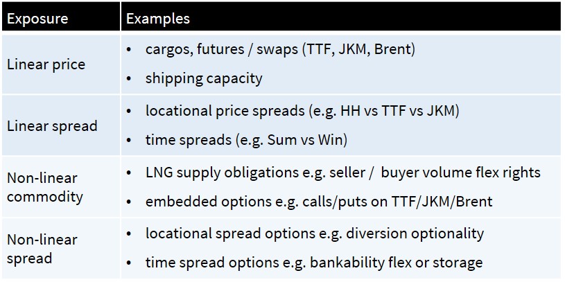
LNG portfolios can be simplified using market price ‘nodes’ and asset ‘exposures’. Market prices act on exposures to drive portfolio value. Diagram 1 shows a simple illustration of key LNG market price nodes. Diagram 2 summarises some key LNG portfolio exposures.

Diagram 1: An illustrative representation of key LNG price nodes

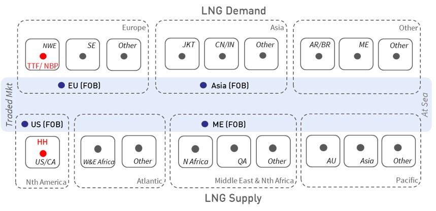
Table 1: Breakdown of some key LNG portfolio exposures

Source: Timera Energy

An effective analytical representation of an LNG portfolio is built on the definition of:

Nodal price dynamics (price level, spreads, correlations, volatility), ref Diagram 1
Portfolio exposures (e.g. commodity positions, asset flex & constraints), ref Table 1.

If you can define a realistic but transparent representation of the way price dynamics act on exposures, you are more than half way to cracking the problem.

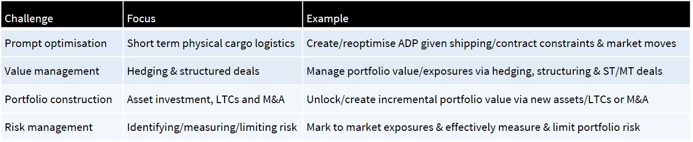
Choosing the right weapon for the hunt

An effective analytical capability to support an LNG portfolio usually covers four distinct areas. These are summarised in Diagram 2.

Source: Timera Energy

There is a natural temptation to acquire an ‘elephant gun’ to tackle all four areas at once. This is a big mistake in our view. There can be common building blocks and a consistent approach, but a ‘one size fits all’ solution ignores the different nature of these four problems.

For example, an analytical tool to support prompt optimisation of portfolio cargo routing & logistics over a 6 month horizon, requires portfolio components & constraints to be represented in very granular detail.

It is ineffective and restrictive retaining that level of detail when analysing value management or portfolio construction over a 2-10 year horizon. Over this horizon, focusing on the impact of commodity price uncertainty is much more important than capturing detailed logistics.

The value of prototyping

Most players in the LNG market are developing their own in-house solutions. This reflects the pitfalls in trying to buy & configure an ‘off the shelf’ solution (as described in the 5 key challenges section above). A well constructed analytical solution can be a unique source of competitive advantage. It can literally pay for itself in a day, via increased value capture.

A key challenge in developing such a solution is effectively defining requirements and approach. It is very hard to do this in a ‘one shot’ upfront design phase. This is where we have found a simplified ‘proof of concept’ can substantially improve results and reduce costs.

The objective of this proof of concept approach is to build a functionally rich and commercially robust working prototype of the enduring analytical solution. This allows:

Practical engagement with business users (e.g. originators, traders)
More effective iterative definition of requirements & methodology
Flagging of any major issues and the flexibility to address these
Early & valuable insight into how analytical results can practically be applied in supporting commercial decision making.

Many elements of the proof of concept can often be efficiently adapted into part of the enduring solution.

For more details on how to tackle the development of an LNG portfolio analysis capability, we have included a link to a briefing pack below.

Briefing pack: LNG portfolio value
Sep 2019 Timera briefing pack with approaches and case studies on identifying & capturing LNG value: Gaining an edge

European gas storage value is recovering

Posted on September 30, 2019January 15, 2020 by David Duncan

Three structural drivers are tightening the gas flexibility balance across Europe:

Rising import dependency: resulting in a reliance on longer & less flexible supply chains (e.g. LNG, Russian pipeline gas)
Power sector transition: with rising renewable intermittency and the closure of nuclear & coal plants increasing the role of gas-fired power plants in providing flexible generation
Ageing infrastructure: investment in new flexible midstream gas assets has ground to a halt over the last 5 years, with owners ‘sweating’ existing assets.

In today’s article we set out clear evidence of a recovery in gas flexibility price signals across 2018-19. We also show ‘backtesting’ analysis that illustrates how price signal recovery is translating into higher value capture from storage capacity.

Price signals recover… at last

The value of gas flexibility (e.g. from storage, production & pipeline flex & regas) is driven by two key market price signals:

Spot price volatility drives the value of deliverability (i.e. flexibility response near to delivery)
Seasonal price spreads drive the value of seasonal flexibility.

Chart 1 shows the evolution of these two price signals since 2016 at Europe’s core TTF hub.

Chart 1: Evolution of day-ahead TTF volatility (left) & front year seasonal spreads (2016-19)

Source: Timera Energy, ICE data

The left panel of the chart shows a clear recovery trend in TTF spot volatility since 2017. Volatility has averaged above 70% so far in 2019 (& is currently above 100% on a 30 day rolling basis). It is interesting to note that this rise in volatility is happening against the backdrop of a well supplied gas market and lower prices. A key driver of higher volatility over the last 12 months has been the role Europe has been playing in absorbing surplus LNG cargoes to balance the global market.

The right panel of Chart 1 shows the forward TTF summer/winter spread as it evolves in the lead up to each storage year (Apr to Mar). A rise in seasonal spreads can arise from three situations: (i) an increase in winter prices, (ii) a fall in summer prices and (iii) both of these factors combined.

Fears around winter tightness are the most common cause of rising spreads. But in 2019 the focus has been on summer price weakness, given a requirement to clear high volumes of LNG imports. This caused the Sum-19 / Win-19 spread to surge across Q1 2019. And the recovery in spreads has also fed through into Sum-20 / Win-20 price spreads, which are around 2.3 €/MWh, almost double the levels of last year.

It is worth noting that price signal recovery at the UK NBP has been sharper given the impact of the retirement of Rough storage in 2016.

Storage margins follow suit

It is no surprise that price signal recovery has translated into higher potential returns for storage capacity holders. Although the level of storage margin capture for any given capacity owner depends factors such as inventory levels and forward hedge positions.

In order to provide a simple benchmark on value recovery we have ‘backtested’ margin capture for a generic fast cycle (60 day cycle) and seasonal (180 day cycle) storage asset. The results across each of the last 4 storage years are shown in Chart 2.

Chart 2: Backtest of margin capture for fast cycle (left) and seasonal (right) storage assets

Source: Timera Energy

We use our in-house storage modelling framework to do this, applying a commonly used rolling intrinsic trading strategy. This involves analysis of margin capture from actual (or ‘outturn’) market price movements where hedges are adjusted against available forward contract prices as these evolve.

Fast cycle margins have recovered by a proportionally higher amount than seasonal asset margins. This reflects the leveraged exposure of fast cycle assets to the recovery in volatility. But there has also been a significant increase in seasonal asset value capture across the last two years, as both volatility and spread recovery lifts returns

Who will benefit from value recovery?

In the short term, the benefits of rising storage margins have been skewed towards capacity buyers e.g. trading desks. This is because buyers have bought storage capacity from asset owners at price levels that reflect the weaker market conditions that preceded the recent price signal recovery.

A continuation in storage value recovery should increasingly flow through to asset owners (vs buyers). This is because increasing volumes of storage capacity are being sold on an annual (or shorter term) basis, as long term contracts roll off and are not renewed.

However the ability of storage owners to maximise value capture depends strongly on capacity sales strategy, contract structures and business model. We explore these factors alongside drivers of continuing storage value recovery in a recent briefing pack (link below).

Briefing pack: European Gas Storage Value
Sep 2019 Timera briefing pack on gas storage margin recovery, market drivers & commercial implications.: Gas storage value recovery

German & Dutch CCGT value case

Posted on September 23, 2019January 15, 2020 by David Duncan

Between 2005-10 there was a mini boom in CCGT investment in Germany and the Netherlands. These projects reached FID against a backdrop of relatively healthy gas-fired generation margins (spark spreads). But by the time CCGTs were commissioned, owners were confronted by a relentless decline in margins.

Renewable penetration gathered pace eroding CCGT load factors. Large new & efficient coal plants also came online, with falling coal and carbon prices increasing the competitive advantage of coal vs gas plants.

But the most pronounced value hit for CCGTs came from the erosion of electricity demand as a result of the global financial crisis. With CCGTs on the margin in most markets, falling demand translated directly into falling load factors & margins.

CCGT values & spark spreads plumetted across 2010-15. But margins started to stabilise in 2016 as gas for coal plant switching gathered momentum. The last 12 months have seen further CCGT margin improvement as European hub prices plummeted. And capacity mix changes over the next 3 years point to a more structural margin recovery.

Today we summarise what we think is an interesting contrarian investment case in existing German & Dutch CCGTs, targeting a 10 year horizon.

Gas for coal switching has driven margin recovery

Between 2010 -2015, relatively low coal & carbon prices underpinned a structural variable cost advantage of coal plants over CCGTs. Clean spark spreads were negative, even on a peak basis, as shown in Chart 1.

Chart 1: Peak German Clean Spark Spreads & current forward curves

Source: Timera Energy, ICE

As a result CCGTs, many of which were newly commissioned, were effectively demoted to a peaking backup role.

The 2016 slump in gas prices started a recovery in sparkspreads and CCGT margins. This margin recovery reversed to some extent across the first three quarters of 2018 as gas prices rose again. But since Q4 2018 there has been a further sharp increase in CCGT generation margins, with plants running predominantly baseload across Summer 2019.

The volatile nature of spark spreads illustrates why it is tough to build an asset investment case on market price views alone. So are there other structural drivers supporting CCGT margin recovery?

Sweeping NW European capacity closures

The German power market is facing almost 25GW of regulatory driven plant closures over the next 3 years. This is a combination of closure of the nuclear fleet and closure of hard coal & lignite to meet Coal Commission targets.

But Germany is not unique. Coal & nuclear closures are a theme across NW Europe. Chart 2 provides a summary of of cumulative regulatory driven closures across NW Europe. These numbers are large: 30GW by 2022, more than 60GW by 2030 (and this does not include ‘end of life’ closures of ageing CCGT plants).

Chart 2 Cumulative regulatory driven closures of NWE coal & nuclear plants

Source: Timera Energy

The scale of closures over the next 3 years will significantly tighten the German and NW European power market balance. Gas-fired plants are set to take up the slack, transitioning to dominate the setting of marginal power prices. In other words, capacity closures will structurally increase gas-plant load factors.

Building a CCGT investment case

There is a well-worn narrative as to why investment in NW European CCGTs is a bad idea: ‘Renewables deployment erodes margin… Decarbonisation risk is growing… Margins are volatile & commodity price dependent… And look at the writedowns owners have suffered over the last 5 years!’.

All of the elements of this narrative are undeniably true. But an asset investment case depends on the relationship between risk adjusted returns and asset acquisition cost. A strong consensus narrative is typically reflected in asset prices.

So let’s turn the problem on its head and approach it by defining a set of 5 drivers that could underpin an investment case:

Motivated sellers: Utilities have taken CCGT writedowns. They are also strategically shifting business models away from owning thermal power assets. Relatively new assets have transacted for cents in the dollar (vs build cost).
Buying optionality: CCGT acquisition can be thought of as buying spark spread optionality. After a tough decade, this optionality is now back ‘in the money’, reducing the risks & costs of value capture. This optionality means asset owners are long volatility… in an environment of rising renewables & structurally tightening energy & capacity balances.
Barriers to entry: Retaining existing CCGTs is the cheapest form of incremental system flexibility (outside specific applications for short duration batteries). The biggest margin threat for existing CCGTs is new CCGT build… but the investment case for new CCGTs just gets tougher as decarbonisation risks grow.
Defined timeline: Plant closures over the next 3 years are not a hypothesis – they will almost certainly be implemented (with German efficiency). That underpins a clear 5 year margin recovery case & target payback window. It is easy to under-estimate further optionality & upside value beyond this (e.g. via introduction of explicit or implicit capacity payments).
Decarbonisation: It is brave to bet against decarbonisation given the current policy momentum in Europe. Yet the more action accelerates, the faster the closure of coal and the bigger the hurdles to new CCGT build. Over a 5-10 year horizon, CCGT owners are long decarbonisation.

Now to dampen all the enthusiasm with a very practical caveat. Not all CCGTs are created equal – the right flexibility, location & plant cost structure are key to making the numbers work.

Inter-market shock roils power, TTF & JKM

Posted on September 16, 2019January 15, 2020 by David Duncan

In our snapshot column last week we flagged a huge rally in power & gas forward curves. The move was driven by three announcements that surprised bearishly positioned markets last Tuesday.

The most important of these was EDF flagging potential new safety issues with its French nuclear fleet. Markets may have short memories, but not short enough to have forgotten the nuclear fuelled fireworks of Winter 2016-17.

Reinforcing the gas market impact of the EDF announcement, the Dutch government further tightened the production cap on the giant Groningen field and announced the end of production by mid 2022.

The third surprise came from the ECJ, which ruled that Gazprom access to the key OPAL pipeline into Germany will need to fall back to 50% of capacity.

Price rises and volatility are likely to continue into this week. The US has blamed Iran for a weekend drone attack that has temporarily crippled more than half of Saudi Arabia’s oil production (~5% of global supply). A very volatile front month Brent contract has been trading 10-20% higher than Friday since the market opened today.

3 factors behind last week’s market moves

French nuke risk

EDF has flagged ‘a deviation from technical standards’ relating to welds on the steam generators of some of their nuclear reactor fleet. The initial EDF statement provided little clarity on how many reactors may be impacted and what the timing of any outages could be.

The French nuclear authority (ASN) subsequently announced that at least 5 reactors had been impacted, with a more detailed statement expected from EDF in the coming week. The resulting uncertainty has seen a significant risk premium driven into French winter power prices, although the impact of outages this winter is unlikely to be as dramatic as in Win 16-17.

Groningen cuts

5 years ago the giant Groningen field in the Netherlands was producing more than 40 bcma of gas. Since then the Dutch government has consistently reduced the production cap on the field given increasing concerns over ongoing earthquakes. The cut announced last week caps gas production at less than 12 bcm for the coming gas year. By mid-2022 output will now fall to zero.

Production cuts had already been flagged earlier this year. But last week’s announcement was at the higher end of market expectations. This helped support a rally across the TTF gas curve, although the big surge in gas prices was more focused in Win-19 given the French nuclear issues.

Gazprom OPAL access

The ECJ ruling last week overturns a 2016 decision to allow Gazprom access to up to 80% of the OPAL pipeline that links Nord Stream to Germany. This effectively returns the 50% cap on Gazprom’s use of OPAL, reducing its ability to flow gas via the Nord Stream/OPAL route by 12.5 bcma.

This volume can flow via the Ukraine/Slovakia route instead. So it is unlikely to result in any immediate supply cuts to Europe. But it shifts the balance of negotiating power towards Ukraine for the very important transit agreement talks that are underway. The transit agreement that allows Gazprom to flow gas via Ukraine (one of its 3 key access routes into Europe) is due to expire at the end of this year.

How has this impacted market prices… so far?

The triple shock that hit markets last week is a great case study in the increasing importance of inter-market linkages. In an energy market version of the butterfly effect, the risk of nuclear outages in France immediately flowed through to higher JKM LNG prices in Asia.

The logic? Nuclear outages in France are ‘backfilled’ primarily by incremental CCGT output (both within France and from neighbouring countries). The implied increase in gas demand dragged up TTF prices, with a knock-on impact across other European hubs. This in turn was transmitted to Asian LNG prices which are underpinned by TTF as European hubs support a well supplied global LNG market.

French power prices for the coming winter rose 12% last Tuesday as the risk of rolling nuclear outages lifted the curve. Power market curves across NW Europe were pulled higher in sympathy (e.g. in UK, Belgium, Netherlands & Germany).

The move in gas prices was almost as pronounced, with Win-19 TTF prices rising around 10%. While the price surge at European hubs was focused on the current winter, the whole gas curve moved higher as shown in Chart 1. This was in part due to bearish positioning after relentless price declines across 2019, but was also helped by the Groningen & OPAL announcements which may have more enduring implications for European gas supply.

Chart 1: One day TTF gas curve move (Tue 10th Sep)

Source: Timera Energy

The events of last week were also supportive of the ongoing rally in NW European CCGT margins. French spark spreads showed particular strength, consistent with a rising forward price signal for CCGTs across the coming winter.

5 things to watch going forward

We finish by flagging 5 factors to watch as a result of the 3 announcements last week:

Win 16-17 revisited: Risks for this winter look less extreme than the shocks of 3 years ago, but recent history shows that it pays to be adequately insured i.e. don’t be caught short flex.
CCGT margins: Price moves last week reinforce the recovery in European gas-fired generation margins we wrote about last week. Nuclear outages are bullish for gas asset margins.
Low Cal constraints: The rapid pace of decline in Groningen’s Low Cal gas production is resulting in a rapidly growing requirement for Hi to Low Cal conversion capacity. Any constraints over the next 3 years may cause price divergence.
Ukraine flows: The OPAL decision will cause flow rerouting & may see Ukraine push Gazprom harder in transit talks into year end. Any disruption of flows via Ukraine this winter will now have a bigger impact.
Gas market balance: Higher CCGT burn & Groningen cuts support Europe’s ability to absorb surplus LNG across next 1-2 years. This may help with the rebalancing of the global LNG market from its current state of oversupply.

In addition there is the wildcard impact of the Saudi attacks on the oil market. Oil is not as direct a driver of European gas & power markets as it used to be given the rapid reduction of oil-indexation in gas contracts. But a disruption of this scale in the oil market will introduce both upward price pressure and volatility to the gas market. Winter 19-20 is shaping up to be anything but boring.

Major shifts in German power pricing dynamics

Posted on September 9, 2019January 15, 2020 by David Duncan

Renewable output is growing fast across North West European power markets. Wind & solar output in Germany accounts for more than 30% of demand. Include other renewables (e.g. hydro & biomass) and this share rises to more than 40%.

Rising renewables penetration is resulting in an increasing number of periods where thermal plants are completely displaced in the merit order. During these periods, power prices can temporarily plunge to low or even negative levels as other forms of lower variable cost capacity set prices (e.g. nuclear, biomass or wind).

Despite rising price volatility associated with intermittency, CCGT and coal plants remain the dominant driver of power prices across NW Europe. Even with a 40% renewable market share in Germany, thermal plants are setting the power price most of the time (sitting on the margin above wind & solar output in the stack). This is particularly evident in the very strong forward curve relationship of power prices versus gas, coal & carbon prices.

It is this forward curve relationship that we look at today. Some major shifts in the relative costs of gas & coal plants in 2019 are having an important impact on the evolution of power prices and generation margins. These are in turn causing a shift in competitive balance and generation asset returns.

4 charts tell the story

Spark and dark spreads are a benchmark for the generation margins for CCGTs and coal plants respectively (power price minus variable cost). These spreads provide an important insight into power market pricing dynamics.

The top two panels in Chart 1 show Baseload & Peak German forward Clean Spark Spreads (CCGT margins) in Germany across the last 18 months. The bottom two panels show Base & Peak Clean Dark Spreads (coal plant generation margins). The 3 lines on each chart show:

Light blue = Summer 2019
Grey = Winter 2019/20
Darker blue = Summer 2020

Chart 1: Base & Peak German CSS (top 2 charts) & CDS (bottom charts)

Source: Timera Energy

Winter

CCGTs are the dominant setter of marginal power prices across the winter. This is reflected in a relatively stable CSS level (grey line in the top panel). As gas prices have declined over the last 12 months, CCGT variable costs have fallen and this has fed through into lower power prices. In other words, falling gas prices have been dragging power prices lower.

The bottom panel show how falling gas prices have also been hurting coal plants. Lower power prices are feeding through into lower CDS, with Baseload Win 19-20 CDS falling by 50% since Q4 -18 (from 8 €/MWh to just above 5 €/MWh). Coal plant load factors and margins are following suit.

The ‘market’ CDS shown in Chart 1 do not include coal transport costs, which further reduce achieved dark spreads. These vary by asset, but range from 2 to 8€/MWh.

Summer

Lower gas prices across summer periods have seen coal plants relegated to a peaking role. This is reflected by a relatively stable Peak CDS across Sum-19 and Sum-20.

The influence of higher variable cost coal plants supporting summer prices has been good news for CCGTs. The top two panels show a big recovery in CCGT generation margins across summer periods as gas prices have fallen across the last 12 months. Lower gas prices are translating into higher CCGT load factors and higher margins.

At the start of Q4-18, Baseload CSS was deeply negative (- 7 €/MWh for Sum-19, – 12€/MWh for Sum-20). Even Peak CSS was hovering around zero. In other words CCGTs were structurally ‘out of the money’ on a forward price basis.

Since then Baseload CSS has surged into positive territory, with Peak CSS rising to around 8 €/MWh for Sum-20 (yes that’s with a positive sign in front of it!). In other words CCGTs are structurally back ‘in the money’ across both next winter and summer.

What does this mean going forward?

We use Germany to illustrate spread and price formation dynamics as it sits at the core of the interconnected network of North West European power markets. But the same dynamics are impacting neighbouring market (e.g. France, Netherlands & Belgium).

The shift that has taken place in relative fuel prices means that power prices across NW Europe have become more strongly linked to gas prices, and less influenced by coal. This reinforces the importance of the gas market in understanding power price dynamics.

The other dynamic that is occurring, almost under the radar, is a significant recovery in CCGT margins in NW Europe. After almost a decade of margin erosion and asset writedowns, CCGTs are in the money again.

The CCGT value recovery story could have more to run. There are some important structural drivers that are set to support CCGT load factors and margins over the next 3-5 years. We will address the evolution of CCGT value soon in a follow up article.

Building a viable battery margin stack

Posted on September 2, 2019January 15, 2020 by David Duncan

We flagged a ‘take off’ in European merchant battery investment as one of our 5 surprises to watch out for in 2019. Investment momentum has been accelerating as the year progresses, and merchant business models have become the dominant focus.

Investment in Europe is being led by the UK and German power markets, with high renewables penetration and a more constructive policy environment supporting battery projects. Merchant investment is being fuelled by a combination of utilities (e.g. EDF, Uniper, Centrica), funds (e.g. Gresham House & Gore Street) and a range of renewables investors looking to pair batteries with solar, wind & other innovative strategies.

But battery investors all face a common challenge: building a viable margin stack that will underpin a return on capital. This is significantly more challenging for battery projects than for renewable or conventional thermal asset investments because of:

Margin sensitivity to rapidly changing market & regulatory conditions (e.g. capacity mix changes & policy evolution)
The complex nature of battery optimisation, across different markets and time horizons, to capture wholesale market margin
A lack of historical data on achieved battery margin performance

One of Timera’s key focus areas this year has been working with battery investors on quantifying robust margin cases. In today’s article we outline our view on how to approach the analysis of a viable margin stack.

Breaking battery margin into buckets

The complexity of battery margin capture means it is imperative to develop a way for investors to understand margin build up, without requiring a double PhD in maths & physics. In our view, the best way to achieve this is to break margin down into buckets as shown in Chart 1.

Chart 1: Battery margin buckets & capability required to capture value

Source: Timera Energy

Base margin: The merchant margin stack is underpinned by non-wholesale market margin streams. These include system services (e.g. frequency response, reactive power), capacity payments and project specific site/locational benefits. The advantage of these margin streams is that they are typically less risky than wholesale market margin and may even support some project debt.
Structural price shape: Power markets have a structural intra-day price shape driven by the variable costs of different capacity types setting prices across the day. A lower bound for battery wholesale margin can be generated based on arbitrage of this structural intraday price shape e.g. via a simple rolling intrinsic strategy. Rising renewables penetration and retirements of coal / nuclear / CCGT plants is acting to increase price shape over time, supporting value in this bucket.
Structural volatility: The very fast reaction speed of batteries in response to price volatility underpins battery wholesale margin capture. There is an inherent underlying level of prompt price volatility (or ‘price noise’) in power markets caused by fluctuations in load, wind and solar. This is increasing with renewables penetration. Value capture is riskier and more complex than for simple arbitrage strategies, but there are formulaic or algorithmic methods to ‘harvest’ value from this volatility without incurring high risk.
Additional volatility: The final margin bucket is made up of riskier extrinsic value. This depends on how much additional price volatility occurs in the market above the inherent ‘price noise’ in bucket 3. Drivers include periods of market tightness and market events such as weather shocks & outages. The amount of value captured here has a stronger dependence on trading capability & commercial judgement.

Interpreting the margin buckets

The portion of value that sits in each of the four buckets varies significantly by commercial strategy, project configuration, location and market. The levels achievable in buckets 1 to 3, determine how much margin must be generated via the higher risk bucket 4, in order to meet required return on capital.

These buckets are very useful in building up a ‘digestible’ view of battery margin analysis. But they are not a way to side step what is a very complex analytical problem behind. The wholesale margin buckets 1 – 4 can be shown separately on a diagram, but are in practice co-dependent. Value is captured via an all-inclusive optimisation of battery flexibility across multiple time horizons. So what analytical tools are required to do this justice?

Quantifying margin bucket value

Firstly, it is important to specifically capture wind, solar & load uncertainty within the market modelling process. It is imperative that these factors are properly simulated (e.g. 500+ simulations) in order to understand their impact on market price volatility.

This means applying a stochastic power market modelling framework (follow the link for an explanation). Traditional ‘Base / High / Low’ scenario analysis of power prices is not appropriate for quantifying battery margins. This approach tends to underestimate both battery value capture and market risk.

Secondly, it is important to model battery margins using a robust stochastic battery optimisation model. This is a separate tool from the stochastic market model. It captures optimisation of battery dispatch against wholesale market prices, including the variable cost impact of battery cycling degradation and bid/offer spreads.

A robust market & margin modelling framework underpins an understanding of how batteries can practically create margin. More importantly it helps quantify the risk dynamics around projected margins.

3 new members join our growing Timera team
Jon Brown joins us from EDF, Steven Coppack from Total & Tommy Rowland from Smartest Energy. As with all of our team members, they have a strong practical background in commercial analytics from their industry roles. More details on Steven, Jon & Tommy on Our Team page.Timera Energy also move into new offices this week: L12, 30 Crown Place, London EC2A 4ES – details here.

Asian LNG demand stalls in H1 2019

Posted on August 26, 2019January 15, 2020 by David Duncan

For several years we have framed the evolution of the LNG market supply & demand balance around one key driver: Asian demand growth. The ability of the market to absorb more than 100 mtpa of committed new supply across 2015-21 depends on Asia. But Asian demand growth has stalled in 2019.

2019 and 2020 are the peak delivery years for the current wave of new liquefaction projects. Global LNG supply has risen by around 12% in H1 2019 (vs H1 2018). But Asian demand growth has ground to a halt (down 0.2% H1 2019 vs 2018). The Latin America & MENA regions are not helping either, with demand contracting by 21% across the same period (after strong 2018 growth).

That leaves Europe having to absorb the full brunt of incremental LNG supply volumes. This is why LNG imports into Europe have surged this year, with hub prices have been pushed down towards Henry Hub support levels.

What happened to Asian demand growth?

Chart 1 shows the evolution of Asian, Latin American and MENA LNG demand since 2016.

Chart 1: Non-European LNG demand

Source: Timera Energy

Across 2016 and 2017, Asia looked to be on a high demand growth trajectory, led by China. Asian demand was absorbing new liquefaction output as well as pulling flexible LNG supply from Europe (particularly across winter).

Chart 1 shows the steady progression of growth in demand from Winter 15/16 to Winter 17/18. But demand growth weakened into Winter 18/19 and has continued to stall in 2019. It is no coincidence that this has happened at the same time as a sharp decline in Asian and European gas prices since Sep 2018.

Table 1 shows the breakdown of demand in H1 2018 vs H1 2019 as well as % changes.

Table 1: Demand breakdown H1 2018 vs 2019

Source: Timera Energy

Four of the big 5 buyers (Japan, Korea, Taiwan and India) had negative growth (H1 19 vs 18). Chinese demand grew at 21%, but this is only around half the demand growth rate China was experiencing in 2016-17. 50% demand growth in the smaller emerging Asian markets is impressive, but is coming off a low base and is relatively low in absolute volume terms.

One of our 5 surprises for 2019 was a drop in global gas demand growth due to weakening economic conditions. That is what is playing out in Asia, exacerbated by tariffs in a growing ‘tit for tat’ trade war that materially escalated last week.

LNG driving the European price snowplough on

LNG that is surplus to Asian, Latam & MENA requirements, is absorbed by Europe’s liquid & price responsive gas hubs. As we set out in July, the growing surplus of LNG flowing into Europe in 2019 is having a ‘snowplough’ effect on the TTF forward curve as shown in Chart 2.

Chart 2: The snowplough continues to roll towards winter

Source: Timera Energy

The very steep front section of the TTF curve reflects market consensus that the current acute oversupply will normalise as demand picks up into this winter. Recovery is being helped by some output curtailment in late summer e.g. Cheniere’s maintenance outages at Sabine Pass and Corpus Christi.

But as evidence of soft demand & weakening economic conditions has continued to emerge across this year, Winter 2019/20 prices have also been declining. Negative Q2 economic growth in Germany and the UK and looming recession fears across Europe are not helping.

Weak prices now… sharper 2020s recovery?

The cyclical nature of the LNG market is underpinned by 5 year lead times for new liquefaction projects. Final Investment Decisions (FIDs) on LNG projects coming to market now were taken in the first half of this decade in a relatively tight post-Fukushima market. But only a small volume of new FIDs were taken across 2015-2017. Even 2018 FID volumes were relatively low, dominated by the large Shell Canada project.

2019 is shaping up to be a higher volume year for FIDs, with Exxon’s Golden Pass and Andarko’s Mozambique projects already approved. But current market conditions may cause some investors to hesitate or delay on 8-10 other LNG projects that are targeting FID over the next two years. A recovery of European and Asian gas prices this winter will be an important factor here.

Asian LNG demand growth may have stalled in H1 2019, but this is a temporary phenomenon. Supply growth is set to remain strong through 2020 and into 2021, so sluggish demand over this period may see a continuation of weak price conditions.

But beyond 2021, the impact of the liquefaction investment hiatus from 2015-17 kicks in. In other words committed new supply growth is likely to fall behind global demand growth on a run rate basis. It is this period from 2022-24 that could see a tight market if FIDs are delayed over the next year or two.trend.

Evolution of UK balancing flexibility

Posted on August 20, 2019January 15, 2020 by David Duncan

Billions of pounds are being invested in flexible peaking capacity in the UK, as the coal fleet closes and older gas plants retire. The two dominant technologies being deployed are gas reciprocating engines and shorter duration lithium-ion batteries.

Only a small volume of this new peaking capacity currently operates in the UK’s Balancing Mechanism (BM). But the BM is set to become the primary driver of value for both engines & batteries across the 2020s.

In today’s article we look at what types of capacity are currently competing in the BM to provide flexibility services. We also look at how this is likely to evolve given capacity mix changes across the next 5 years.

Why will the BM be so important?

Margin capture for UK engines and batteries is currently focused on:

‘NIV chasing’: forecasting cashout prices & trying to run imbalances to capture margin accordingly (see here for article on battery challenges in chasing cashout prices)
Triads: running in periods of peak demand to help reduce supplier charges
Ancillaries: providing services such as STOR, frequency response (e.g. FFR) and fast reserve

Step forward five years and it is likely that BM value capture will dominate all of these sources of margin capture for most peaking assets. But why such a rapid margin transition?

Market participants increasingly recognise that NIV chasing is a dying game. Average system imbalance volumes in the UK are typically only several hundred MWs. Yet there will soon be GWs of flexible capacity chasing relatively small imbalances. That will increase forecasting errors & risk and reduce returns. The practice of intentionally running large imbalance volumes into gate closure is also likely to attract the attention of regulators, who may implement rule changes to disincentivise this.

Margin from triads and ancillaries is also declining. Triad revenue will largely disappear by 2021 as a result of policy changes already announced. And increasing competition to provide frequency response, STOR and fast reserve services has been driving down returns for these balancing services.

The combination of these factors means the future for flexible peaking capacity is likely to be focused on capturing value in the BM and prompt forward markets (e.g. Day-Ahead and Within-Day markets).

Balancing Mechanism 101

The BM is the mechanism that the system operator (National Grid) uses to balance the UK electricity market in real time. Market participants that are registered as ‘BM Units’ can submit bids and offers in the BM, reflecting prices at which they would be prepared to flex down or flex up respectively.

National Grid then uses a combination of these bids & offers as well as other balancing services contracts to ensure the system balances in real time. This task is becoming more challenging over time as wind & solar intermittency increases. But that is also creating increasing opportunities for flexible assets to capture margin in the BM.

An important distinction between the BM and the wholesale market is that all participants are ‘paid as bid’ not paid the price of the marginal provider of energy. This in combination with volatile prices, means that there can be some very lucrative opportunities in the BM, during periods of system constraint.

The flip side of very volatile prices is a relatively high level of volume risk. Capacity owners do not know when they place bids & offers whether they will be accepted or not. Therefore value capture in the BM often has a significant opportunity cost linked to foregone margin from the wholesale market.

What capacity provides BM flex & how will this change?

Flexibility requirements in the BM can be summarised as:

Flex up: the ability to provide more energy to the system (or reduce demand)
Flex down: the ability to reduce output onto the system (or increase demand).

Chart 1 provides an illustrative scenario of the evolution of the percentage of different technology sources providing Flex up volumes across 2020-25.

Chart 1: Provision of flex up volume in the BM

Source: Timera Energy

Flex up is currently dominated by CCGTs. Increased output can either come from ‘spinning’ units that can achieve an incremental top tranche of output (e.g. CHP), or by starting an idle unit. Coal units have also historically been active in providing flex, but weak dark spreads and high start costs are undermining their ability to compete with CCGTs. Hydro and pump storage also provide some flex.

Looking forward over the next 5 years there are likely to be some substantial changes. Coal will disappear and older CCGTs close. At the same time, the volume of flex provision from both gas engines and batteries is likely to rapidly increase. Engines have very low start costs and high ramp rates. Batteries are almost instantaneous in their ability to flex output.

Chart 2 provides an illustrative scenario of the evolution of the percentage of different technology sources providing Flex down volumes.

Chart 2: Provision of flex down volume in the BM

Source: Timera Energy

CCGTs again dominate provision of flex down currently. This is typically provided by spinning units reducing output to minimum stable generation levels (incurring an efficiency loss) or switching off altogether.

Wind curtailment is also playing a growing role. The reason for this is that high wind output (particularly in northern regions) is increasingly causing Grid to take balancing actions to alleviate transmission constraints (to flow power south). The least cost way to resolve these constraints can be to curtail associated wind output.

The volume of flex down services provided by gas engines and batteries will be impacted by the role of wind curtailment. But there are also other considerations e.g. flex down is more difficult for engines to provide than flex up, because of the relatively low load factors at which units run.

Peaking unit transition to the BM

Transitioning to focus on BM value capture adds complexity to the peaking asset business model. Portfolio scale and a strong commercial & analytical capability are important ingredients of developing a competitive presence in the BM. Without these, individual assets will likely only earn a fraction of the ‘theoretical’ modelled value available in the BM.

Peaking asset owners can try and sidestep scale & capability overheads by outsourcing flex management to a third party (e.g. Centrica, Orsted). But the contract haircuts for BM value capture are typically high.

BM value capture is a different game to triads and ancillaries margin, where flex asset owners could negotiate with third party providers to capture the lion’s share of available margin. The balance of power sits firmly with the service provider for BM value capture. This is because it is significantly higher risk and higher return, with the ability to generate value underpinned by a robust trading & analytical platform.

We have written previously about a more challenging margin capture environment driving further aggregation & consolidation of UK peaking assets. Business model transition to focus on BM margin capture is set to reinforce this trend.

Will European gas prices recover or ‘snowplough’?

Posted on July 15, 2019January 15, 2020 by David Duncan

Time for a simple thought experiment. If you had a ‘one shot’ chance to gaze into a crystal ball and see the evolution of one energy market driver over the next two years, what would you choose?

European gas pricing dynamics would be at the top of our list.

Despite rapidly declining hub prices in 2019, a nascent recovery in the value of gas supply flexibility is taking place, as seasonal price spreads and spot price volatility recover. But hub price evolution is not just important from the perspective of the European gas market.

European gas pricing has an extended influence across other markets and value chains. For example:

Global LNG supply: LNG pricing in a well-supplied market is currently being driven by TTF. So European gas price levels will have a strong influence on FID decisions for new supply projects shaping the next wave of LNG supply into the mid 2020s.
Coal plants: Low hub prices in 2019 have driven coal plant cashflows deep into the red across Europe. If this environment continues into 2020-21, it may cause the accelerated economic driven closure of large volumes of European coal plant capacity.
Renewable investment: Merchant renewable investment is in the early stages of evolution in Europe (e.g. solar projects in Spain). Cost declines are one factor, but power price levels have become a much more important revenue driver. Gas hub price levels are now the primary driver of power prices across Europe and will be an important factor determining how fast merchant renewable investment gathers pace.

Alas we have no crystal ball. So instead, in today’s article we consider 5 key drivers likely to shape the evolution of European gas pricing dynamics.

The recovery versus ‘snowplough’ question

Some unusual and interesting price dynamics have been evident in the European gas market in 2019. Spot hub prices have been in a relentless decline across the first half of 2019. This sits in stark contrast to the steep rise in prices across the first part of 2018, as can be seen in Chart 1.

Chart 1: Global gas price benchmarks

Source: Timera Energy

The primary factor explaining the difference between the path of hub prices into summer 2018 vs summer 2019 is the LNG market. 2018 saw flexible LNG diverted from Europe to meet robust Asian LNG demand. In 2019 a pronounced temporary oversupply in the global LNG market has seen surplus cargoes flooding into Europe.

If you consider the TTF forward curve to be the closest thing we have to a crystal ball, curve shape is consistent with a sharp recovery of prices into the coming winter. But as 2019 has progressed, the front of the forward curve has steadily been pushed lower (at least until the beginning of July which we will come to in a minute). Think of a snowplough steadily cutting into a bank of snow.

Summer 2019 prices started the year above 16 €/MWh. By the beginning of Jul-19 prices had fallen almost 40% to 10 €/MWh as shown in Chart 2.

Chart 2: Snowplough effect at the front of TTF curve

Source: Timera Energy

As Sum-19 prices have fallen at the front of the curve, an ever steeper spread has opened up to Win-19. The market has been pricing in an acute but temporary oversupply of gas across the current summer.

This is the result of surplus LNG flowing into Europe, unusually low storage injection demand and falling coal prices (dragging down power sector switching levels). As Q2 progressed, Winter-19 prices also started to show some signs of weakness (see Jul-19 vs Mar-19 curves in Chart 1).

Then last week saw a sharp rebound in European hub prices, with front month TTF now rising more than 25% since the start of July. This move has caught a very bearish market off guard. Prices of other commodities have also moved sharply higher as global central banks have reaffirmed efforts to try and stimulate growth and inflation.

Price moves like this are driving TTF spot price volatility higher in 2019. But is the ‘July jump’ in prices just noise or the start of an enduring recovery into winter and beyond?

We look next at the five factors we think will determine whether European hub prices recover (as suggested by the forward curve) or continue to ‘snowplough’ (as in Chart 2)?

5 key drivers to watch

LNG demand growth

The strong pick up in surplus LNG flowing to Europe since Q4-18 (shown in Chart 3) is a function of new LNG market supply temporarily outstripping demand growth. Chinese demand continues to grow, although forward contracting has meant Chinese buyers have been less active purchasing spot cargoes. But LNG demand from the rest of the ‘Big 5 Buyers’ club (Japan, Korea, Taiwan & India) is significantly lower in 2019 than 2018. Demand is also down from Latin American and Middle Eastern buyers.

Chart 3: European LNG sendout & the TTF vs Asian spot price spread

Source: Timera Energy

We raised a red flag recently on the potential impact of global economic conditions on gas demand. The trade war appears to be having a particularly strong impact in weakening manufacturing and industrial output. The evolution of LNG demand over the next 1-2 years will be a key factor determining how much surplus LNG will flow into European hubs.

Ramp up rate of new LNG supply

The other side of the LNG market equation is supply. The highest volumes of new liquefaction capacity from the current supply wave are scheduled to come online across 2019 and 2020. But evidence over the last three years has shown that there is significant uncertainty around project delays and ramp up rates.

A number of other projects commissioned across 2015-19 have experienced up to 12 month delays in reaching full output. There have also been unexpected outages. Seasonal production volume dynamics, where output is significantly higher across the colder northern winters, add to supply side volume fluctuations.

European power sector switching levels

The main mechanism for the European gas market to absorb incremental LNG flows is coal for gas plant switching in the power sector. This means that European hub prices are influenced by coal and carbon prices.

One of the factors causing downwards pressure on TTF in 2019 has been falling coal prices (carbon prices have remained relatively strong). This has been pulling down the switching range (that we track in Chart 1) across Q2 2019, which in turn weighs on gas hub prices.

The switching range acts as an anchoring point for European hub prices. Spot prices may temporarily deviate from this range, but the TTF forward curve is strongly linked to switching levels. Keep a close eye on the evolution of coal and carbon prices to understand how this switching range evolves.

European gas demand

European economic growth has slowed sharply in 2019. Manufacturing and industrial output are particularly weak, with Germany leading the decline. The probability of a recession in 2019 or 2020 has risen significantly.

It is unclear:

how much economic weakness will impact gas demand in Europe and
how much of this impact is priced into the TTF market forward curve (recognising growing bearish sentiment across H1 2019).

It is worth keeping an eye on the evolution of European economic growth and gas demand data.

European pipeline supply

Russian flow volumes to Europe hit a new all time high in May 2019, following on from April’s record LNG import volume. Norwegian import volumes have been strong. There has even been a slight recovery in North African imports.

Will pipeline imports remain this strong into winter? Gazprom has not shown any signs of flow sensitivity to low prices yet in 2019. There is however a heavy maintenance schedule on the NCS across the next two months which will temporarily impact Norwegian flows. Market expectations are for strong flow volumes to continue, but any deviation from this (e.g. Russian pull back or major outages) could have significant price implications.

Implications for value of European gas supply flex

After a tough five years, midstream gas asset value is coming back into focus in 2019. Regas terminal utilisation levels have jumped and pipeline flows have been strong. But the most interesting asset class is gas storage.

Seasonal price spreads in 2019 have surged higher, as the front of the TTF forward curve has declined. More importantly for storage asset value, spreads are recovering further out on the forward curve also. Sum 20 to Win 20 TTF spreads have risen above 2.20 €/MWh, with NBP spreads stabilising above 10 p/th.

TTF and NBP spot price volatility have also been steadily rising across 2019, with the ‘July jump’ in prices adding fuel. Conditions of higher volatility and spreads are typically associated with periods of market tightness and rising prices. It is an encouraging sign for storage capacity value that price signals are recovering despite the well supplied, low price environment.

We will be taking our usual summer break from feature articles until mid August. In the meantime we will continue to publish material via our Snapshot and Angle columns on the Blog Home page.

FX movements driving energy prices

Posted on July 8, 2019January 15, 2020 by David Duncan

Global trade & geo-political tensions have been steadily rising this year. For example the US-China trade war (& broader power struggle behind this), US-Iran tensions and Brexit. In parallel, the monetary policy measures of central banks are becoming increasingly unconventional and aggressive (e.g. negative interest rates & structural quantitative easing).

These dynamics are likely to play out in the form of rising currency volatility or even larger scale currency shocks. In this environment it is a good time to consider the impact of FX movements on energy prices.

The EUR-USD relationship is key

The primary driver of currency movements impacting European energy markets is the EUR-USD FX market. This is the world’s most liquid market with in excess of 1 trillion USD daily transaction flow.

Global commodity markets such as oil and coal are traded in USD terms. So if the EUR falls against the USD, commodity costs rise in EUR terms. This has a direct impact on assets exposed to oil, liquids & coal prices. Chart 1 provides some context on the evolution of the EUR-USD exchange rate.

Chart 1: EUR-USD price chart over last 5 years

Source: barchart.com

Interest rate, inflation & economic growth differentials between the US & Europe play an important role in driving EUR-USD levels. The EUR has fallen against the USD since the start of 2018, as interest rates & growth in Europe have been lower than in the US. But the EUR has stabilised in 2019 as US growth has slowed and financial markets have priced in US rate cuts across H2 2019 (Eurozone rates are already negative).

European gas prices & FX movements

The impact of FX movements on European gas prices is more complicated. European gas prices are driven by the TTF hub and essentially priced in EUR terms based on the prevailing supply & demand balance across Europe’s interconnected hub network.

While European gas is priced in EUR terms, coal to gas switching levels are an important marginal driver of hub prices. This creates an implicit USD linkage via the variable cost of coal plants. If the EUR rises against the USD, it reduces the variable cost of coal plants, putting downward pressure on relative switching levels and TTF.

LNG spot prices & FX movements

The impact of currency movements on LNG prices is also more dynamic. LNG is traded in USD terms. But European gas hub prices underpin LNG spot pricing dynamics. So even though cargos change hands in USD, it is TTF (a EUR based market) that is the global spot price benchmark.

If for example the EUR appreciates against the USD, the TTF price level typically rises in USD terms (as can be seen via TTF futures contracts transacted in USD/mmbtu). That in turn can pull up Asian spot price levels which are typically traded on a ‘variable cost plus’ basis to TTF.

There is also a further currency driver that is important to consider given current oversupplied conditions in the LNG market. TTF prices have been driven down towards US Henry Hub ‘shut in’ levels by surplus volumes of LNG flowing into Europe. So TTF is currently effectively trading on a ‘variable cost plus’ basis to Henry Hub.

The current role of Henry Hub as a global spot price floor therefore introduces a USD price linkage to both European hubs and Asian LNG spot prices.