Defending energy portfolios against a credit event

Posted on October 12, 2015January 16, 2020 by David Duncan

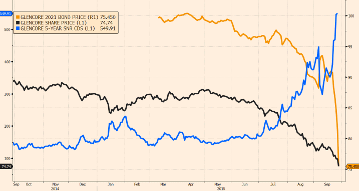
Last week we looked at the threat of a systemic credit event in energy markets. Market prices are flashing a warning signal about the capitalisation and interrelated exposures of a number of large commodity trading firms.

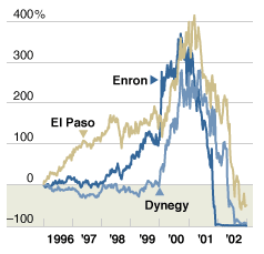
However you assess the imminence and magnitude of the current threat, historical evidence shows a clear track record of systemic credit events. We looked at the 2001-03 Enron collapse last week as a case study. The events at the peak of the financial crisis in 2008-09 are another example. So rather than waiting to see if ‘commodity traders 2015-16’ is the next occurrence, what defensive preparations can be made in advance?

Issues with credit risk management in energy companies are often rooted in the basics. For example:

Ensuring the robust definition & measurement of credit exposures
Making sure these are reflected in commercial decision making and the ongoing management of counterparty exposures.

Credit risk management problems are often driven by an under-resourcing of credit risk functions, given the perception that they are just a cost centre or administrative control function. There can also be challenges within large energy companies when it comes to managing credit risk within business units (e.g. trading functions) versus the management of broader corporate credit exposures.

On a day to day basis credit risk may appear relatively dormant compared to market risk. But every once in a while it rears its ugly head and the scale of losses can dwarf those of more closely regulated market risk exposures. This means that credit risk is all about robust and efficient practices that provide a structural defence. Ramping up a focus on credit risk once a credit event is already in motion smacks of closing the stable door after the horse has bolted.

Defence in two steps

Building a basic defence against credit risk can be broken down into two key parts: (i) measures in place at the time of transaction and (ii) measures taken on an ongoing basis during the life of the contract.

Time of transaction: Company credit policies should dictate which companies are permitted counterparties, and (via a system of exposure limits) to what extent. Within this policy framework, the application of a Credit Value Adjustment (CVA) ensures that credit risk is priced into transactions on a deal by deal basis. CVA is calculated on the simple principle that a buyer of poor credit standing gets charged more than a strong buyer.

The CVA attempts to quantify the appropriate credit risk premium (or discount, when buying – recognising that credit risk is symmetrical in forward exposures). Its use is twofold:

As a direct input into contract pricing
As the basis for an internal transfer (actual, into a credit reserve; or notional for management accounts) to provide ‘self-insurance’ against the statistically expected losses arising from the portfolio.

Additionally, an extension of the CVA calculation generates an ‘at-risk’ number (sometimes called ‘CVaR’). CVaR is used in assessing how much of a credit limit is utilised by a transaction, and how much risk capital is represented by the deal. CVA is becoming common practice in energy companies, helped by an increased regulatory focus (e.g. IFRS 13).

Ongoing management: On a continual basis through the life of the contract, various practical steps are taken to update the calculation of, minimise, and manage the ongoing exposure. This exposure may actually be getting worse with time, as market conditions and/or general corporate weakness affect the counterparty adversely and call their commercial performance into question.

These steps include clearing, netting, bilateral margining and calling for collateral. Importantly they typically depend on the contract being written with good credit support terms.

Ongoing management of credit risk also falls back on robust definition, measurement & reporting of credit exposures. This requires an effective capability to analyse the future evolution of credit exposure, for example incorporating techniques such as:

Potential Future Exposure (PFE): quantification of maximum expected credit exposure of a contract/portfolio for a given time horizon & confidence interval.
Credit VaR (CVaR): quantification of default loss for a given time horizon & confidence interval.

These techniques are the building blocks of tracking and managing credit risk on both an individual contract and a net portfolio basis. The stochastic measurement of PFE for an example hedging contract is illustrated in Chart 1.

Chart 1: PFE measurement example

Source: Amsterdam Complexity

Direct hedging: In addition to these steps Credit Default Swaps (CDS) also provide the ability to directly hedge exposures to larger counterparties. But these are less commonly used by energy companies to manage day to day contractual credit risk. This is in part due to the complexities associated with exposure matching, pricing and management of CDS in relation to the underlying credit exposure.

Backing up principles with practicalities

The defensive steps described above make for a good routine credit risk management discipline. But energy companies face a number of practical problems in implementing these. For example:

Default data: The analytical techniques outlined above (e.g. CVA, CVaR) require default data and other inputs that typically come from rating agency assessments. The 2008-09 crisis is riddled with examples of how rating agency analysis was found wanting (e.g. their analyses of capital adequacy). We would be surprised if similar issues did not arise during the next major credit event.
Default measurement: Even good-quality default data understate credit/performance risk in a commercial sector like energy because they relate to bond default, and companies fail to perform under ordinary commercial contracts before (if ever) they default on bonds.
Structural change: Many energy contracts have very long tenor, more so than in other industries. Looking back at events over the last decade (e.g. commodity supercycle, shale gas, financial crisis, Fukushima) illustrates that even ten years is a very long time. Structural changes in the industry over several years can systematically undermine the creditworthiness of large players or even whole sectors at a time.
One shot defence: Although the credit support tools exist for inclusion in contracts, it is surprising how often companies fail to bolster their long-term contracts fully or allow credit terms to be negotiated away. There is generally only one opportunity to do this justice.
Heritage: Some energy companies come to traded-market credit risk management from a retail/utility heritage. This can result in relative weakness and under-resourcing of credit risk management versus e.g. market risk management.

Common sense over black boxes

Analytical techniques such as CVA, CVaR & PFE can materially improve an energy company’s defence against major credit events. But relying too heavily on these tools can be dangerous as was illustrated in 2008-09.

Probabilistic methods to measure and price credit risk need to be applied in a transparent manner rather than as ‘black box’ number generators. Outputs also need to be challenged with a healthy degree of scepticism. If results cannot be demonstrated to company management via simple benchmarks & sense checks then it is likely that the methodology is the problem rather than the audience.

This leads to a final key element of credit risk management: stress testing. Systematic and carefully designed stress-test scenarios are vital in a regular, periodic programme of stress tests. Stress testing is a specific discipline with best practices of its own, but it is particularly relevant in credit risk management. A few obvious examples:

What is the impact of the default of your largest counterparty (or top 3; or a sector of counterparties with interconnected exposures e.g. commodity traders)?
What is the impact of counterparty default on key contracts, either from an individual asset or portfolio perspective?
If 1. and 2. seem mundane then ‘reverse engineer’ a scenario that causes major portfolio stress.
If unable to raise a sweat with 3. it is probably time to use a bit more imagination.

The creditworthiness of large commodity traders is likely to ebb and flow with the fortunes of commodity prices and broader credit market stress. But there is enough smoke on the horizon to justify a prudent review of credit risk management. In our view building a robust defence is about effective policy, CVA analysis & implementation and contract credit support at the time of transaction. Then on an ongoing basis this needs to be backed up by the measurement and management of credit exposures, bolstered with appropriate stress tests.

Authors: Nick Perry, David Stokes, Emilio Viudez Ruido

Watch out for a major credit event

Posted on October 5, 2015January 16, 2020 by David Duncan

It is often said that when the tide goes out on commodity prices we find out who’s been swimming without shorts on. The market smells trouble brewing amongst some large commodity trading companies. The most prominent of these, Glencore, has attracted plenty of attention over the last week. Since the latest commodity rout began in August, Glencore’s share price has slumped and the cost of insuring default risk has soared.

The focus on Glencore is partly because of its size, but also because it is one of the few publicly listed commodity traders. This means that there are much clearer market price signals for balance sheet stress. But Glencore’s exposure to falling commodity prices is far from unique. In fact the majority of global commodity traders have a similar business model. That means that trouble for one is likely to signal trouble across the sector. These companies are big energy market players and that brings credit risk sharply into focus.

For the energy industry, the echoes of Enron’s collapse in 2001 are sufficiently loud that they are worth revisiting. In this article we look at the credit risk issues that are rapidly evolving in the current market. But we do so in the context of looking back at the Enron driven credit event as a case study for what may happen next. We will then return next week and consider what’s to be done about it from a credit risk management perspective.

What’s all the worry?

Glencore and its commodity trading peers, companies such as Vitol, Trafigura, Noble & Mercuria, have evolved their business models substantially over the last 10-15 years. Growth has been fuelled by a big bull market in commodities. As an example, Vitol (the world’s largest oil trader) had zero profit in the late 90s but ballooned to a $2.28bn profit by 2009.

Commodity traders have expanded their core trading business by backing it with large asset portfolios in an attempt to claim margin across the supply chain. This has meant business model evolution has been accompanied by an expansion in structural long portfolio exposures to commodity markets. The theory of this business model is that the trading business manages portfolio risk via hedging core exposures, i.e. the companies are essentially a margin business that should benefit from market volatility.

But current market price signals suggest that this theory may be harder to implement in practice. Chart 1 shows the prices of Glencore’s shares and bonds plunging in September. At the same time Credit Default Swaps (CDS) have risen sharply. Last week’s CDS prices meant that traders required about 14 percent upfront to protect against a Glencore default over the next 5 years. That is the highest level since April 2009 during the midst of the financial crisis.

Chart 1: Glencore market price signals

Source: FT

Glencore is not alone. The shares of another large publicly listed commodity trader, Noble Group, have also fallen sharply over the last two months. Stress is also evident in non-listed companies via traded debt prices. The yield on Trafigura’s 2018 bonds soared to over 10% last week (from yields under 5% in early August) reflecting a sharp increase in credit risk premium. The threat of credit contagion echoes the events around Enron’s demise last decade and this is a useful case study to revisit.

Enron: A credit event case study

Enron was a major force in commodities trading beyond its dominance of gas and power markets. However Enron was not actually a victim of falling commodity prices. In fact, Enron had gone significantly short (and profitably so) in key markets during the commodity price declines that preceded its collapse. It was not even finished off by the major scandals that later engulfed its senior management. The fundamental cause of Enron’s demise was one of the oldest problems in business: it was under-capitalised, with profits greatly outstripping cash-flow. That may turn out to be a problem that Enron’s successors confront during the current commodity downturn.

The knock on credit risk impact of Enron’s balance sheet issues are very relevant to current events. Enron was everybody’s counterparty. This was frequently through Enron Online, a universally used B2B platform (with Enron as principal in every trade) unmediated by exchange or clearing. But it was also via large structured contract positions, often relating to underlying physical energy assets. Despite this Enron was never rated above BBB+.

As Enron’s balance sheet stress grew, the dominos fell, but in slow motion, which was:

initially confusing, disguising the very real sector-wide capital weakness, but
helpful in allowing the banks to manage what might otherwise have been an avalanche

The other energy merchants remained in a state of denial and envisaged picking up Enron’s market share between them. But they were all, to a greater or lesser degree, also undercapitalised. One by one, at the rate of approximately one per month, other energy merchants went bust, the last big one being TXU Europe in 2002 a year after Enron filed for Chapter 11 bankruptcy. Chart 2 illustrates the speed of the energy merchant downfall.

Chart 2: Rise and fall of the energy merchants

Source: Thomson

Many of these collapses were accelerated by (i) the complex chain of credit exposures, and (ii) softening of energy prices from 2000 onwards, especially power prices. For example Enron’s disappearance had a significant negative impact on TXU Europe. AES Drax was primarily hedged by TXU. Then when TXU Europe went under, and as UK power prices fell sharply, AES Drax also went under (as did a significant portion of UK IPPs, and British Energy).

This is a key takeaway from the Enron experience relevant for current market events. The Enron episode exemplifies not only Credit Risk but Systemic Risk, when feedback loops cause an entire commercial infrastructure to come under enormous strain, causing a credit event that impacts a significant number of industry players.

A further systemic consequence was a huge hit to the then-booming Project Finance sector in banking. At the turn of the century there were well over 70 banks actively engaged in the energy sector. This fell to a dozen or so by 2003. The fall of a key player that is heavily engaged with an entire market can have devastating consequences, within and beyond that market.

Returning to 2015

Glencore and its peers are big enough, and in sufficiently similar positions, to suggest 2015 may evolve into a large-scale credit risk event. The interconnected nature of commodity trader exposures suggests that systemic risk is also a threat. The low interest rate environment over the last 5 years has added to this threat. Cheap borrowing costs have incentivised commodity traders to issue debt and utilise structured finance opportunities which bring capital into focus as margins decline.

How would the commodity sector, and more specifically the energy sector, cope with such a credit event? The fact that the industry has been tested by (i) the Enron collapse and (ii) the financial crisis credit shock of 2007-09, suggests that lessons have been learned. Credit risk management techniques have improved, although these are often far from adequate as we will explore in more detail next week.

What feels uncomfortable this time is that wide spread commodity price weakness is happening against a backdrop of weakening global growth and tightening corporate credit conditions. Banks were well placed to manage liquidation of large portfolios and take over bust IPPs after the Enron crisis, but are less so now. US oil producer debt is an accident waiting to happen as we have set out previously. These conditions increase the likelihood that one or two large failures trigger a systemic credit risk event. The UK is particularly vulnerable to a systemic event in the commodity sector given the importance of resources companies to the FTSE indices.

Even if systemic risk is avoided right now, at the very least we can expect commodity trading companies to come under intense capital pressure. This means drawing in their horns and taking out risk-capital and liquidity from the market. And that will have negative consequences for all market players, even those which are adequately capitalised and have well-managed portfolios.

Article written by Nick Perry & David Stokes.

Gas flex case study: the impact of losing Rough storage

Posted on September 28, 2015January 16, 2020 by David Duncan

Investment in gas supply flexibility is supported by two key market price signals. Summer/winter price spreads drive investment in seasonal flexibility and short term (or prompt) price volatility drives investment in deliverability. Both price signals have declined significantly this decade choking off investment in new supply flexibility.

As well as a dearth of new asset investment, owners of existing assets are unwilling to invest in renewal or life extension capex in existing assets. In March this year, Centrica announced a 25% reduction in available working volume at its Rough gas storage site. It appears that this capacity may now remain offline, given the challenging investment economics associated with rectifying Rough’s well integrity issues in the current weak spread environment. SSE’s 33% reduction of withdrawal capacity at its Hornsea site is another recent example of lost flexibility due to poor market returns.

It is reasonable to hypothesise that the issues at Rough may not just be limited to a 25% capacity reduction. Over time, the incremental capex spend required to maintain the remaining working volume may present a similar challenge. In this article we explore what the loss of Rough means in a UK context as well as considering the potential market price impact.

The loss of Rough is used as a case study in this article. A solution may be found for the current well issues, particularly if there is a timely recovery in seasonal spreads. However a similar logic applies to the retirement of other ageing flexible infrastructure in North West Europe (e.g. significant loss of Groningen flexibility).

Rough storage in a UK context

The full effective working volume of Rough, prior to the onset of well integrity issues, was around 3.8 bcm. This represents about 80% of the UK’s 4.7 bcm of total storage capacity working volume. In working volume terms Rough represents the lion’s share of UK storage capacity as illustrated in Chart 1 which shows UK storage utilisation across the most recent gas year.

Chart 1: UK storage capacity utilisation 2014/15

Source: National Grid

The restrictions announced by Centrica in Mar 2015 reduced Rough working volume by about 1 bcm. Compression has been maintained such that the maximum deliverability rate from Rough is unchanged. However the reduction in working gas means on average the UK market will have around 6 mcm/day less withdrawal capability across winter.

The medium range storage facilities in Chart 1 are predominantly fast cycle salt cavern facilities (e.g. Aldborough & Holford). The configuration of these fast cycle assets is skewed towards fast injection & withdrawal rates. This means they pack much more punch in deliverability terms than Rough, but need to re-inject fairly regularly to maintain working gas levels. The short range stocks in Chart 1 consist of LNG tank storage assets. These play a relatively minor role in contributing to UK supply flexibility given low volumes and LNG supply chain logistical constraints that curtail flexibility (e.g. managing boil-off costs & the requirement to clear the tanks for additional cargoes).

Chart 1 gives a sense of the significance of a scenario where Rough is phased out completely over time. When measured against current operational storage capacity, such an outcome would reduce UK working gas volume by around 80% and deliverability by around 25%. Storage is complimented by other sources of supply flexibility through the Norwegian pipeline network and UK interconnectors. But by any measure the loss of Rough is a big deal.

The market impact

Seasonal price spreads of 15-20 p/th are required to support investment in large scale seasonal storage (e.g. depleted offshore fields). Yet the NBP summer/winter spread has steadily declined this decade to levels around 5 p/th today as shown in Chart 2.

Chart 2: NBP front year summer/winter spreads

Source: Timera Energy

We have written previously about how this is driven by dynamics across the European gas market rather than factors that are specific to the UK market. Weak demand and an overhang of flexibility have crushed seasonal spreads across all European hubs, with little anticipation of a recovery priced into the forward market. Chart 3 shows a comparison of seasonal prices and price spreads at Europe’s two major hubs: TTF in dark blue and NBP in light blue.

Chart 3: Current NBP vs TTF forward prices and spreads (24th Sept 15)

Source: Timera Energy

Chart 3 shows that NBP and TTF prices broadly converge on a forward basis over summer. But in winter periods, the UK NBP trades at a premium to attract the necessary imports from the Continent that are required to support seasonal demand. This means higher seasonal spreads at NBP (5 p/th or 2.40 €/MWh) than at TTF (2.9 p/th or 1.30 €/MWh). These dynamics do not necessarily hold on a within-year basis where prices can flip and spreads can rise as the result of specific supply & demand issues (as was seen in Summer 2014 when the renewed flow of LNG imports pushed summer prices down).

The forward spreads in Chart 3 illustrate the issue that Centrica faces in investing life extension capex into the Rough facility. Selling seasonal storage capacity at 5 p/th (plus a small extrinsic value premium) is an uninspiring task. Yet the loss of Rough capacity and other European gas supply flexibility (e.g. loss of flex from the Groningen field in the Netherlands) does not appear to be reflected in market pricing.

The only historical data point for loss of Rough capacity is the outage period following the fire in Feb 2006. Seasonal price spreads surged and spot volatility approached 300%. But it is difficult to compare market conditions in 2006 to today. Large volumes of flexible UK gas supply infrastructure were commissioned across the 2007-10 period (e.g. the Langeled pipeline, new fast cycle salt cavern capacity and a substantial increase in LNG regas capacity) which has to some extent reduced the UK’s dependence on Rough.

Even so, the loss of Rough would certainly impact market pricing. The UK gas market would become much more dependent on importing flexibility (e.g. from Norway and through the interconnectors). This would mean more pronounced price signals to attract gas flows i.e. higher NBP spot volatility and some increase in seasonal spreads. The UK would also be much more susceptible to winter price shocks, with more frequent and prolonged price jumps likely required to attract incremental LNG imports.

If Rough were to close it is not at all clear that market price signals would support investment in a large replacement seasonal storage facility. Seasonal price spreads at NBP are to a large extent driven by interconnection with the Continent which is oversupplied with seasonal flexibility. Instead peak deliverability constraints in the UK would drive much more pronounced prompt volatility. And the supply side response would likely come in the form of fast cycle not seasonal storage.

Vattenfall’s German sale: mixing lignite & water

Posted on September 21, 2015January 16, 2020 by David Duncan

Vattenfall is kicking-off a formal sales process to dispose of its lignite and pump storage hydro assets in Germany. The sale will result in a significant change in asset ownership in Europe’s largest power market. The larger Czech and Polish coal generators (e.g. CEZ, EPH and PGE) have the most obvious interest. But there should also be interest from within Germany as well as from new entrants further afield (e.g. strategic Asian investors and funds).

The share prices of E.ON and RWE illustrate the challenges of owning generation assets in Germany. Power plant values reflect current depressed levels of German generation margins. These have been battered by a three pronged onslaught of falling coal prices, rising renewable output and weak demand.

But generation investment is cyclical in nature. For prospective buyers, Vattenfall’s assets represent a means to gain a large but relatively cheap foothold in the German market. And unlike Centrica, which pulled its recent UK CCGT sale, Vattenfall has a clear mandate to sell these assets regardless of price expectations.

The sale of Vattenfalls’ German lignite assets (summarised in Chart 1 below) has been a story that is at least two years in the making. The sale has been delayed by a lack of clarity around a new German climate levy which has threatened the early closure of some lignite assets. As a deal sweetener Vattenfall has also lumped in more than 2.5 GW of predominantly pump storage hydro assets.

Chart 1: Vattenfall lignite plants & associated mine production

Source: Vattenfall

This mix of lignite and hydro provides an interesting case study in the evolving margin dynamics of flexible German power assets. The value drivers for lignite & pump storage generation are very different. Yet both asset types share a common exposure to the impacts of renewable penetration which are acting to transform the German power market.

Price behaviour in the German power market

We have previously written about German power market pricing dynamics. But in summary, the formation of marginal power prices is predominantly driven by hard coal plants. With coal on the margin, the fortunes of power prices have been closely linked to steadily declining global coal prices as shown in Chart 2.

Chart 2: German front year baseload power (vs. Netherlands & Nordpool)

Source: Vattenfall

The power price decline in Germany has been exacerbated by two consecutive years of mild weather and associated weak demand. Demand fell 3.8 percent in 2014 despite the fact the German economy grew 1.4 percent. But these conditions have exposed some natural support for power prices around the 30 €/MWh level, as the variable cost of lignite assets acts to support prices in periods of weak net system demand.

The other important factor driving lower power prices has been a rapid increase in renewable output. This has acted to create downward pressure on both:

The absolute level of power prices, as the supply stack shifts right and lower variable cost plant are pushed on to the margin
Within-day price shape, given higher daytime wind & solar load factors which act to flatten peak prices

The impact of the first of these factors is a key concern for lignite assets. Whereas the value of pump storage assets depends heavily on the second. Chart 3 illustrates some of the effects in play via a plant type breakdown of German generation stack output.

Chart 3: German generation output in Week 36 2015 (1^st week of September)

Source: Energy Charts

The chart illustrates the scale of the impact of swings in output of wind (light green) and solar (yellow). Hard coal can be seen setting marginal prices during weekdays (with CCGTs completely out of merit). The last two days shown in the chart illustrate a weekend period with weak net system demand (low demand + high wind). In these situations hard coal is pushed out of merit with lignite plants providing marginal price setting flexibility. The within-day peak shaving role that pump storage plays can be seen via the light blue output range.

An alternative view of the German supply stack ordered by plant type & variable cost is shown in Chart 4.

Chart 4: German supply stack tranches (2014)

Source: RWE

This chart illustrates the ranges of generation capacity that set marginal power prices under different conditions in the German market. The majority of time periods sit within the black tranche of hard coal. But in periods of high renewable output and weak demand (as shown in Chart 3), less efficient lignite plants can set marginal prices. In periods of low wind & solar output and high demand, CCGTs come on to the margin, driving up system prices and lignite plant returns.

Lignite and pump storage value dynamics

The primary exposure of lignite plants is to the absolute level of the power and carbon prices. But through power prices, lignite assets also have an important secondary exposure to European coal prices (given coal plants dominate marginal price setting). Fuel costs on the other hand are much more within the owners control given adjacent lignite mines.

It is useful to contrast the margin dynamics of lignite vs hard coal assets. Chart 5 illustrates the evolution of German hard coal plant margins (CDS). Despite the substantial 2010-15 fall in power prices shown in Chart 2, hard coal plant margins have been fairly resilient as result of coal plants role in setting power prices. In other words falling power prices reflect falling coal prices, de-risking hard coal generation margins.

Chart 5: German peak and baseload clean dark spreads (CDS)

Source: Timera Energy

Lignite plants do not benefit from this fuel vs power price correlation benefit. But they do have the significant benefit of being the lowest variable cost producers in the German power market. And that ultimately acts to protect plant load factors and cashflows.

Pump storage assets are a different prospect. Value is driven by the flexibility to respond to price shape (intrinsic value) & short term price volatility (extrinsic value). In addition there are significant revenue streams from provision of transmission/ancillary services. These value drivers are summarised in Chart 6.

Chart 6: Pump storage value drivers

Source: Timera Energy

Renewable penetration is dampening price shape which negatively impacts the value of storage. But intermittency is driving volatility and price spikes (both up and down) into prompt prices. This increase in prompt volatility is an important structural trend that is a consequence of increasing intermittent generation.

These factors mean energy margin is transitioning from the intrinsic to the extrinsic value buckets shown in Chart 6. Quantifying and capturing this value comes down to understanding the practical constraints around optimising & hedging pump storage cycling optionality.

Battery storage represents a long term threat to pump storage margins. But cost and regulatory issues are likely to mean battery storage penetration is gradual at best. It could be a long time before battery storage rollout (currently measured in MW not GW) approaches anything near the scale of Vattenfall’s pump storage assets.

German regulatory environment

The delay in Vattenfall’s sales process reflects the regulatory risk associated with the German power market. Policy issues are not the focus of this article. But it is worth summarising three factors which will have an important impact on Vattenfall’s assets:

Emissions policy: A proposed climate levy that could have caused the closure of a number of older lignite plants was officially scrapped in July 2015. But the German Energy Minister is sticking by a target for 40% GHG reduction by 2020. Lignite plant are a key source of these emissions, so uncertainty remains as to how policy measures to deliver this target may impact plant lives going forward.
Capacity payments: A refinement of the German power market design is currently underway (Electricity Market 2.0). Particularly important are the mechanism(s) that will be adopted for remunerating flexible capacity as renewable penetration increases. Latest indications favour a more minimalist approach focused around energy market price signals. But a capacity reserve has been announced for 2.7GW of Germany’s oldest lignite plants which will be paid to provide back up and then closed by 2020.
Renewable support: Despite plummeting wholesale prices, Germany has the second highest power bills in the EU (after Denmark). While there is still broad popular support for the Energiewende, it remains to be seen to what extent consumers may start to push back on the rising costs of continued renewable expansion.

These factors appear to represent a formidable landscape of policy threats for German generators. But the government’s recent climate levy back down was an important signal. The large German utilities are facing very serious balance sheet issues. These are being exacerbated by liabilities associated with the nuclear generation fleet that is planned to be phased out by 2023. There is likely to be some important regulatory downside protection from the fact that it is in no one’s interest for the German government to cripple the incumbent utilities.

Vattenfall portfolio investment case

The value of German lignite assets comes down to the evolution of power prices and therefor hard coal prices and dark spreads. The current depressed price and spread environment is forcing generators to close an overhang of gas and older coal fired plants. There are GWs of capacity in the German market that are unable to cover costs at current market prices.

While a coal price recovery may not be imminent, long term downside is likely to be limited by the fact that global prices are at or below the long run marginal cost of new mines. Lignite asset downside is also supported by their position as the lowest cost thermal producers in the generation stack. Building an investment case turns on getting comfortable with asset margin downside while recognising the value of asymmetric upside from recovering prices and spreads.

Pump storage assets are much less exposed to the absolute level of power prices. Instead it is decreasing price shape and increasing prompt price volatility that are the key value drivers. The renewable penetration that is eroding thermal asset margins, is supporting an increase in short term price fluctuations and within-day price spikes. Pump storage asset value comes down to the practical capture of extrinsic margin associated with this prompt volatility.

The Vattenfall assets provide a means to build a sizeable position in the German market (or enter the market in scale). But the foundation of an investment case will be built around buying a portfolio of low variable cost flexible assets in a depressed price environment. History tells the story of the cyclical nature of power asset investment. It also provides evidence of healthy returns from investing in low cost quality assets during the trough of the cycle.

Article written by David Stokes, Olly Spinks & Emilio Viudez Ruido.

Structural transition in gas prices

Posted on September 14, 2015January 16, 2020 by David Duncan

A sharp slump in spot gas prices last summer marked the start of a new phase of global gas pricing. This summer the gas market has been relatively quiet. Instead price action has been focused on the oil market. After recovering back towards 70 $/bbl in Q2, Brent plunged back under 50 $/bbl in August, pointing to a more prolonged period of oil price weakness.

An emerging oversupply of LNG and weak oil prices have seen the re-convergence of global gas prices. But so far European spot gas prices have remained broadly in line with oil-indexed contract prices. We have not yet seen a repeat of the global gas glut conditions of 2009-10, where a gap opened up between the cost of oil-indexed supply and hub prices. But this may change over the next to years.

The state of play

Chart 1 shows the rapid re-convergence of European & Asian gas prices over the last 12 months. The precipitous decline in Asian prices has been driven by the combined effect of (i) LNG oversupply and (ii) falling oil prices dragging down oil indexed contract prices.

In fact the last 12 months resembles 2011 in reverse. It so far remains to be seen if the gas glut dynamics of 2009-10 are to follow.

Chart 1: Global gas price evolution

Source: Timera Energy

As summer winds to an end, European hub prices are hovering around the 6.00 $/mmbtu level. Asian spot LNG is changing hands at around 7.30 $/mmbtu (Japanese marker). So the acute pressure on European hubs from weak Asian LNG prices has temporarily subsided from earlier this year when the Asian vs European spot price spread briefly inverted.

But Europe’s status as the LNG market of last resort (or global gas sink) remains. European hubs are currently providing key support for global gas prices. Even if LNG is not flowing to Europe, it is being priced off a basis to European hubs.

There is no doubt as to the predominant exposure of large suppliers and portfolio players. The LNG market is long gas against a backdrop of relatively weak demand from Asian utility buyers. Rather than much anticipated demand from China driving price recovery, Chinese buyers are looking to unload portfolio length.

The main buying interest in the LNG market is currently focused on Middle Eastern buyers. But the competitive nature of the current Egyptian and Jordanian supply tenders and the likelihood of small premiums over NBP prices illustrates the LNG supply overhang.

After a brief recovery in Q2, oil prices are declining again, pointing to further downwards pressure on long term gas contract prices into 2016. The lagged impact of the oil price recovery on Asian contract prices can be seen via the red-dashed Asian LNG price proxy in Chart 1.

Higher slope coefficients on Asian LNG contracts mean contract prices fall faster in response to weakening oil than European pipeline contract prices. This also means that the Asian LNG market may transition to a role of dragging European hub prices lower, rather than pulling them higher.

Asian LNG contract prices are likely to end 2015 below 7.50 $/mmbtu (given the lagged impact of crude prices). Prices are set to fall further next year if oil price weakness continues. Lower Asian LNG prices are likely to drive the increasing diversion of flexible supply from Asia to Europe. This is the reverse effect of the post Fukushima period and means more LNG flowing into European hubs.

Looking forward into 2016

No crystal ball is required to predict the trend of supply in 2016. There is more than 50 bcma of new liquefaction capacity entering the LNG market across 2015-16. A number of large liquefaction projects will be commissioned from late 2015 into 2016 e.g. the two remaining Australian export projects on Curtis Island, the first US export trains at Sabine Pass and the expansion of the giant Gorgon field off Western Australia.

This new supply needs to find a home in a market that is already long LNG. To date there has been a notable absence of opportunistic buying in response to lower prices. China is the most important candidate, but weak manufacturing and export data and central authority devaluation of the yuan do not bode well for a significant pick up in Chinese import demand in the near term. That points to large volumes of new supply flowing into European hubs, either directly (e.g. from Sabine Pass) or indirectly (e.g. via Australian gas displacing other Asian imports).

We have written previously about the risk of breaching the ‘tipping point’ in the European gas market. This is the point where the contractual flexibility to ramp down oil-indexed pipeline swing contract volumes to make way for LNG imports is exhausted. Once past the tipping point, oil-indexed prices are pushed out of their current role as the dominant setter of marginal hub prices. In turn, spot prices may need to fall significantly to induce demand response from gas-fired power plants e.g. in a 4-6 $/mmbtu price range. Conditions in 2016 look like they could well test this theory.

Gearing up for battle

From a European supplier perspective, it is not the absolute level of gas prices that are the key driver of portfolio value. It is rather the differential between the cost base of long term oil-indexed contract supply and hub prices which drive sales revenue. The divergence between oil-indexed and hub prices in 2009-10 precipitated big supplier losses and a round of supply contract re-negotiations & concessions that continued until 2012-13.

Suppliers have so far been shielded from the pain of 2009-10 given hub prices have remained broadly in line with contract prices. But if hub prices diverge from oil-indexed prices again in 2016, similar pressure on portfolio margins can be expected. A particularly dangerous scenario for suppliers would be a recovery in oil prices at the same time global gas market oversupply intensifies.

After 5 years of pain from power generation portfolio write downs, the balance sheets of European utilities are ill prepared for another shock. This would likely precipitate an intense phase of supply contract renegotiations, portfolio restructuring and asset divestments. It could also be the catalyst for the significant restructuring of portfolio supply to more closely reflect hub prices, with LNG offering a competitive alternative to pipeline supply.

Current market conditions and asset margins point towards a growing likelihood that utilities will need to raise capital to sure up balance sheets. New capital with an appetite for energy assets is waiting in the wings in the form of infrastructure and private equity funds. But fund appetite for merchant risk is limited by conservative risk/return mandates. So transaction structures are likely to involve utilities retaining the lion’s share of asset market risk exposures.

Article written by David Stokes and Olly Spinks

UK spark and dark spreads in animation

Posted on September 7, 2015January 16, 2020 by David Duncan

The evolution of generation margins for gas and coal fired power plants are having wide reaching implications across European gas and power markets this decade. A collapse in spark spreads (gas plant margins) over the last five years has seen CCGT load factors crushed and units closed or mothballed. This has in turn driven a pronounced decline in European gas demand, contributing to weakness in gas prices, seasonal spreads and volatility.

Dark spreads (coal plant margins) remained somewhat stronger until 2014, supported by falling coal prices. But the onset of price weakness at European gas hubs last summer has steadily eroded dark spreads.

Weak gas and coal plant margins are a key issue in the UK power market, with the threat of closure of 8-10 GW of thermal generation capacity over the next two years. The 2GW Eggborough coal plant last week became the latest station to announce it may close next year.

In order to investigate the dynamics of the evolution of clean spark and dark spreads (CSS & CDS), we have animated the evolution of spot vs forward spread curves. The approach we have used is similar to the previous animations we have done for the Brent crude curve and the NBP gas curve.

The reason why we like these curve animations is because they add a new dimension to the analysis of market price dynamics. Industry analysis is often very focused on spot prices. This is understandable given that spot prices drive asset dispatch decisions. But the majority of asset value is typically hedged against forward curve prices. An animation sheds light on:

The relationship between spot vs forward price behaviour

Forward price dynamics along different parts of the curve

And in the case of generation margins, how spark spreads evolve relative to dark spreads

UK Baseload and Peakload spreads are shown in Charts 1 and 2 below. We will come back in a subsequent article to show CSS & CDS animations on the Continent.

Chart 1: UK Baseload CSS & CDS

Chart 2: UK Peakload CSS & CDS

Overview of spread dynamics

It is worth starting with a few observations about UK forward spread dynamics. The dominance of gas fired capacity in the UK power market (which has ~ 25GW of installed CCGT capacity) plays an important role in driving price evolution. Marginal power prices are predominantly set by gas fired plants, meaning there is a strong correlation between gas and power prices.

This provides strong support for Baseload CSS around the 0 £/MWh level and prevents pronounced negative spreads from occurring as seen in Continental power markets this decade (where coal plants set marginal prices). This logic has historically been used by trading desks to support spot vs curve strategies e.g. buying negative forward spreads to deliver into spot on the basis that gas plants on the margin should ensure spreads will be positive on delivery.

The dominance of gas plants in setting marginal prices also means the CSS curve has a less pronounced seasonal shape than the CDS curve. Both gas and power price curves have seasonal shape (which smoothes the CSS curve) whereas the CDS curve has a more pronounced shape given the absence of shape in coal forward prices.

Spread curves are also influenced by the contango (upward sloping) and backwardation (downward sloping) dynamics of the underlying fuel, carbon and power price forward curves. For example, the steep backwardation that can be seen in the UK CDS curve in 2013 is a function of strong coal and carbon curve contango.

But perhaps the most important observation about price behaviour from the animation is that spot spreads have a very strong influence on CSS and CDS forward curves. This is often referred to as ‘the prompt wagging the curve’. We have explored this dynamic in previous articles, but in the UK power market it is also a function of relatively weak liquidity. With the market dominated by vertically integrated utilities, liquidity is normally restricted to the front three seasons (and is often limited within this time horizon).

Coal vs gas plant margin behaviour

From 2011 to 2013, a gap opened up between coal and gas plant margins. This was driven by relative fuel price movements. Across this period, gas prices remained broadly linked to oil (above 100 $/bbl). Whereas the onset of oversupply in the global coal market saw coal prices decline more than 50%.

Coal-fired plants opened up a large competitive advantage over gas-fired plants. This pushed older less efficient CCGTs out of merit, causing the weakening of spark spreads that can also be seen from 2011-13.

Two factors have rapidly changed the fortunes of UK coal fired-plants since 2013:

The carbon price floor has been increased to 18 £/t, adding a substantial carbon cost on top of EUA certificates
NBP gas prices have declined as oil prices have fallen and an oversupplied LNG market has set in

The current forward CDS curve sits barely above the CSS curve. Yet the fixed costs of coal-fired plants (~ 50 £/kW) are roughly double those of CCGTs (~ 25 £/kW). In other words less efficient coal plants are running at negative margins. This is the primary driver of the announced closures of around 5GW of coal capacity in the UK (Longannet, Eggborough, Ferrybridge). While these closures are consistent with the previous UK government’s carbon price floor policy intentions, they are pushing the UK power market into a period of unprecedented capacity tightness.

Spread curves are not pricing in a capacity crunch

If the threatened plant closures materialise, National Grid’s measure of UK system reserve margin is likely to swing into negative territory over the next two winters. The forward market appears remarkably complacent about this.

There was a pronounced contango (upward slope) that developed in the peak and baseload CSS curves through 2012-13. This was in part a function of backwardation in the gas forward curve, but also reflected power prices increasing along the curve in anticipation of the system capacity margin tightening. The animation illustrates how this CSS contango (particularly peak CSS) has been flattened since summer 2014. Again this relates in part to the reversal of NBP gas curve contango, but the current UK forward spread curves are not pricing in any recovery in generation margins despite a looming capacity crunch.

So why is there no market price signal emerging to encourage thermal plants to remain open? If you take a cynical view of UK power market regulation, you can argue that the market anticipate ssome form of regulatory intervention will prevent a capacity crunch come what may. But in our view that is not the whole story.

The number of more speculative trading desks taking an active view on forward UK power price evolution is declining, given capital constraints and the winding down of energy trading functions at banks. This means weaker liquidity along the curve with the forward market dominated by utilities and generators.

These conditions suggest that there is ‘prompt wagging the curve’ logic in play. In practice this is likely to be caused by weaker prompt spreads causing generators to maintain or even increase their forward hedge cover to protect downside exposure, rather than lifting hedges in anticipation of higher margins in the future. As a result the market price signal from the onset of a capacity crunch is likely to be seen first in spot prices and it may happen very rapidly.

Article written by David Stokes, Olly Spinks & Emilio Viudez Ruido.

The next leg down in commodity prices

Posted on August 31, 2015January 16, 2020 by David Duncan

It has not been a peaceful summer in global commodity markets. After a six month period of consolidation, July saw a renewed broad based decline in commodity prices. This has continued through August as concerns over China’s growth prospects have intensified.

Crude oil prices have plunged back through January levels and look set to test the lows set at the height of the global financial crisis below 40 $/bbl. This will in turn put downward pressure on global LNG prices and European gas hub prices as the year progresses.

All eyes on China

All is not well in China, the global engine room of commodity consumption. The country that used more cement in three years than the US did across the entire the 20^th century, looks to be suffering a pronounced economic slowdown.

China devalued the yuan in early August in an attempt to sure up its ailing export sector. This has triggered a new bout of global risk aversion and sharp selloffs in the currencies of other developing markets. It has also been the catalyst for a renewed selloff in commodity prices as fears grow that Chinese demand will weaken going forward.

The surprise yuan devaluation intensified selling pressure in commodities markets. A weaker currency means that raw commodities will be more expensive for Chinese buyers. But perhaps more importantly the devaluation may be a signal of heightened concerns within the Chinese administration as to the state of the export driven economy. The August Chinese Purchasing Managers Index reading (47.8) showed a third consecutive month of contraction. Export data was particularly weak.

The summer commodity price fall can be seen in Chart 1 which shows the benchmark global commodities index (CRB) breaking down through levels reached at the peak of the financial crisis rout in 2009.

Chart 1: CRB Index

Global commodity markets are sliding down the backside of the commodity supercycle price mountain. Chart 1 is an interesting illustration of the short term elasticity of commodity supply. Given the lead time on investment cycles, the supply of resources is typically slow to respond to increases in demand. This is evident in the dramatic price rises that preceded the supercycle peak in 2008 (driven primarily by rapid Chinese economic expansion).

But production response has a habit over overshooting, as well as being slow to respond to market price declines. As Chinese demand projections have been revised down over the last year, producers in most commodity markets have refocused on battling for market share in the face of precipitous price declines.

The oil rout continues

The oil market is a case study in market share warfare. Since OPEC’s aggressive production stance triggered the price decline below 80 $/bbl last year, global production has increased not decreased. US and Gulf state producers have fought to sure up output in the face of lower prices, driving an increase in crude production of 2 million barrels per day. The lifting of Iranian sanctions (expected early next year) is likely to add at least another half a million barrels per day.

It is this increase in production set against a backdrop of weakening demand projections that has fuelled the latest leg down in crude oil prices. Chart 2 shows the US WTI crude oil price benchmark breaking below 40 $/bbl last week to levels not seen since the peak of the financial crisis in 2009. A big short covering rally at the end of the week saw WTI crude close the week above 44 $/bbl, hinting that the sell off may be over done in the short term. But a structural recovery is difficult to see until the current supply overhang dissipates.

Chart 2: WTI crude oil price

When crude was above 60 $/bbl in May, we set out why we thought oil would head back to 40 $/bbl and remain weak for a more prolonged period than the market was pricing in. That logic still holds and we think the US shale oil investment cycle needs to be materially disrupted to cause a stabilisation in prices back towards crude long run marginal cost benchmarks above 70 $/bbl. Look out for some major distress and consolidation amongst US shale producers over the next twelve months.

The implications for global gas pricing

The latest leg down in oil prices is in the process of feeding through into global gas prices. The role that oil-indexed European pipeline contracts play in setting marginal hub prices, ensures a strong relationship to oil, albeit on an approximately six-month time lag. The bulk of the latest decline in oil-prices will not feed through into European gas contract prices until early next year. But suppliers are likely to utilise any available flexibility to delay contract take until these lower prices take effect (as was seen in Q1 2015).

The majority of long term Asian and European LNG contracts are also oil-indexed. But the slope co-efficient of LNG contracts to oil is typically higher than that in European pipeline contracts. The time lag for contract oil-indexation are also typically shorter. This means that there is likely to be a sharper impact of the crude decline on LNG prices, reinforcing the factors driving Asian & European gas price convergence and acting to increase the flows of LNG into European hubs. Lower oil-indexed hub prices and cheaper LNG imports are set to work in tandem to drive down European hub prices.

In the post Fukushima years (2011 to mid-2014) the global gas market was focused on high oil prices and Asian demand driving regional price divergence, supply concerns and a premium to ship gas to Asia. That thesis has undergone a sharp reversal in the space of just 12 months. Now lower oil prices and an oversupply of new LNG production are driving regional price convergence and a downtrend in prices back towards those at the US Henry Hub.

Gas volatility & investment in deliverability

Posted on July 20, 2015January 16, 2020 by David Duncan

The article below is our last before the summer break. We will be back with more in late August.

There are two key structural trends in play that will place increasing demands on the flexibility of European gas supply infrastructure over the next decade:

European import dependency will increase substantially as domestic production declines, increasing the likelihood and impact of supply shocks (e.g. infrastructure outages, supply disruptions)
Gas demand swings in the power sector are set to increase as intermittent renewable output expands

These trends primarily drive a requirement for greater gas deliverability (as opposed to greater seasonal flexibility). Yet the market price signal for deliverability, spot hub price volatility, has remained subdued over the last five years.

In this article we look at the evolution of historical volatility. We investigate the recovery in volatility that started last summer and has since fizzled out. And we explore some of the factors driving ongoing weakness in hub price volatility & the implications for investment in deliverability.

2014: a volatility review

There were several sharp spikes in day-ahead price volatility across 2011-13 relating to specific supply shocks (e.g. the Norwegian field and IUK outages in 2013). But the effects of these were short lived and had little impact on underlying volatility weakness, as illustrated in Chart 1.

Chart 1: The evolution of TTF prompt prices and historical volatility (2010-25)

Source: Timera Energy (using LEBA data)

2014 ushered in the start of what looked to be a shift in the underlying level of volatility. Higher volatility is typically associated with higher prices in energy markets. But the first half of 2014 saw hub prices fall (weak demand, higher LNG imports) and volatility rise, particularly over the summer which is typically a relatively weak time for volatility. As hub prices fell they disconnected from oil-indexed contract prices, reducing contract take and the use of swing flexibility.

Towards the end of 2014 and into 2015, volatility levels sank back towards the depressed levels of the last few years (sub 40% on an annualised basis). Over this period hub prices re-converged with oil-indexed contract prices, due in part to a hub price recovery and in part to falling oil prices. The volatility recovery of summer 2014 proved to be a short lived phenomenon.

What does 2014 tell us about the future?

The factors that drove this rise in volatility are interesting as they may apply again in periods going forward. Warm weather at the start of 2014 caused a slump in demand as we explored in detail last week. As the summer approached gas hubs were swamped with heavy storage withdrawals and an increase in LNG imports due to weak Asian spot prices. This knocked the market out of equilibrium and drove hub prices well below oil-indexed contract prices. Prompt volatility rose as a result.

2014 gas demand was 52bcm down on 2013, given some of the warmest weather in recorded history. In other words it represented a low demand outlier event. But the other factor contributing to oversupply, an increase in LNG imports, is something that is set to happen in much higher volume over the next 3 years as new liquefaction capacity comes online.

We have outlined in a number of previous articles the risk of higher LNG import volumes driving the European gas market past the tipping point of available pipeline contract flexibility to absorb them. In an oversupplied market such as this, flexible LNG flows will play an important role in setting marginal hub prices. They will typically do so at price levels below oil-indexed contract prices under similar (or more severe) conditions as those seen in the summer of 2014. It is also likely that lower gas prices will see greater swing demand from CCGT power plants as they come back into merit. In addition LNG imports are likely to ebb and flow in response to short term regional price signals in the LNG spot market.

So while conditions of oversupply have been associated with depressed volatility over the last few years, this will not necessarily be the case going forward. A transition to a more serious state of oversupply may see both LNG imports and the power sector influencing marginal hub prices (as they disconnect from oil-indexed contract prices). And this may drive an increase in prompt price volatility.

Investment in deliverability

Europe also faces the question of how new flexible gas supply infrastructure will be commissioned given the current absence of a market price signal in a weak volatility environment. The same logic applies to the approval of renewal capex spend on ageing existing infrastructure (e.g. Centrica’s Rough facility in the UK), which may have a higher cost structure than deliverability sourced from investment in new flexible assets. Virtually no new deliverability is being added across Europe in the current market environment. In fact the market is losing flexibility from existing infrastructure, e.g. Groningen field cut & the reduction of UK storage flexibility (Rough & Hornsea).

That is not to say there is anything wrong with the European gas market. Just that there is a disconnect between current price signals and the investment in deliverability required into next decade. In that context, if you can buy or invest in high deliverability flexible assets that are priced based on current volatility conditions, you may stand to make healthy returns into next decade.

European gas demand, LNG flow & hub prices

Posted on July 13, 2015January 16, 2020 by David Duncan

Last week we explored the impact of weaker Chinese LNG demand on European hub prices. We set out a scenario that illustrated the impact of European hubs having to absorb higher volumes of flexible LNG as the global balancing market.

This week we shift our focus to European gas demand. We aim to set out why European demand growth will be even more important than Asian LNG demand in driving the evolution of both European hub prices and spot LNG prices over the remainder of this decade.

European gas demand is a big deal

In the last 5 years gas demand across Europe has fallen by a staggering 19%. This equates to a 109 bcm reduction in annual demand from 585 bcm in 2010 to 476 bcm in 2014 (based on the IEA’s definition of Europe’s 32 gas consuming countries).

Putting this 5 year reduction in European demand in the context of the LNG market, 109 bcm represents more than 40% of total current annual Asian LNG demand. Approximately half of the fall in demand over the last 5 years occurred in 2014 alone (52 bcm), the result of exceptionally warm weather, e.g. Germany’s weather was the warmest in recorded history.

From these high level numbers, it is clear that the evolution of European gas demand over the remainder of this decade is a going to be a key driver of the global gas market balance. We will come back to look at the drivers of European gas demand in more detail in a separate article. But it is worth noting a few of the factors behind the decline:

Fall in power sector gas demand as gas plant load factors have declined
Relatively weak European economic growth
Some structural reductions in demand e.g. energy efficiency improvements in residential gas demand (although these are small in size relative to the attention they have attracted)

Of these 3 factors, the power sector (1.) has been by far the largest contributor to the overall reduction in gas demand (once weather influences are accounted for). The fall in demand has been induced both by gas vs coal plant switching (given relatively weak coal prices) and by an increase in renewable output across Europe.

Looking forward, it is important to note the impact of extreme weather in 2014. Industry forecasters have been consistently overly optimistic in predicting a recovery in European gas demand. But it is reasonable to expect a significant demand recovery in 2015 regardless, given normalisation of the weather effects of 2014. This may also be supported by somewhat higher gas plant load factors as the result of weaker gas hub prices.

Demand growth and Europe’s ability to absorb LNG

In order to explore the impact of weaker European demand on hub prices, we use the same scenario framework we set out last week. We have defined what we see as a reasonable weaker gas demand growth scenario over the next 5 years as follows:

European demand recovers by 27 bcm in 2015 as weather normalises, approximately half of the fall in demand from 2013 to 2014
European demand then grows at an average of 0.75% from 2015-2020, primarily reflecting a recovery in power sector demand as the result of weaker gas hub prices
That results in an annual demand of 522 bcma by 2020 (slightly less than the 2013 demand level) & can be contrasted with the more robust demand scenario we set out in April where demand recovered to 562 bcma by 2020

We combine this European demand scenario with an assumption that Asian LNG demand growth continues at a reasonably robust rate (18% CAGR), again as we assumed in the original LNG market scenario we set out in April.

The resulting impact on the European gas supply & demand balance is shown in Chart 1

Chart 1: European gas market balance with 0.75% average demand growth (2015-2020)

Source: Howard Rogers

It is useful to contrast this chart with the one we showed last week. In the weak Chinese LNG demand growth scenario from last week, Europe only really started to struggle to absorb surplus flexible LNG from 2019.

The tipping point (where pipeline contract flex is exhausted), is reached much earlier in a weak European gas demand scenario. This comes down to the scale of European gas demand relative to Asian LNG imports. Asian demand growth is impressive, but it is coming off a much lower base.

The point of the scenario analysis above is not try and forecast a weak demand outcome. Instead we are trying to illustrate that weak demand adds to the challenges Europe is already facing in absorbing growing surplus global volumes of LNG over the remainder of this decade.

Over the last two weeks we have looked at the impact of (i) weaker Asian LNG demand and (ii) weaker European demand on the European gas market balance. Of these two, European demand is the bigger driver. But a combination of the two in parallel would cause a larger and more rapid development of surplus gas at European hubs. The risk of this happening and the resulting impact on hub price dynamics means we are keeping a close eye on the tipping point framework we set out recently as new liquefaction capacity comes to market.

Article written by David Stokes, Olly Spinks & Howard Rogers

European hub prices and Chinese gas demand

Posted on July 6, 2015January 16, 2020 by David Duncan

One of our themes in 2015 has been the increasing importance of the LNG market as a driver of European hub prices. To date we have focused more on the evolution of gas supply. But we turn now to focus on the other side of the equation: gas demand growth.

The global gas price convergence that has prevailed since summer 2014 means there is a strengthening relationship between global LNG demand and European hub prices. This is because Europe is acting as the swing importer of surplus LNG in an oversupplied market. We set out the logic of this relationship in a recent article here.

The weaker global LNG demand growth is, the more LNG that will need to flow into Europe in order to balance the global LNG market. The more LNG that flows into Europe, the greater the downwards price pressure at European hubs.

Growth in global LNG demand over the next decade will be driven by two main factors:

Developing Asian LNG importers (particularly China)
Growth in European LNG imports as domestic production declines

Both these factors will in turn be important drivers of European hub price dynamics. So over the next two weeks we will look at scenarios that explore the impact of:

Weaker Chinese LNG demand growth (this week’s article)
Weaker European gas demand growth (next week’s article)

We do this with the same framework we used for the global LNG supply and demand balance scenario we presented in late April.

China LNG demand dynamics

Chinese LNG demand made headlines in Q1 2015 after suffering its first ever quarterly decline (y-o-y) since China started importing LNG in 2006. This followed LNG import growth data for 2014 (10% CAGR) which was also significantly down compared to previous years, as shown in Chart 1.

Chart 1: Annual growth in Chinese LNG imports

Source: Interfax

This slowdown in LNG demand was consistent with a sharp slowdown in Chinese gas demand growth to 5.6% in 2014. The primary cause has been weakening Chinese economic growth and industrial gas demand. Looking forward, there is also considerable uncertainty over the evolution of Chinese gas demand. Demand growth will be heavily influenced not only by economic growth, but by the pace of a centrally planned push to reduce pollution from coal-fired power production. The level of regulated gas prices will also have an important influence on demand.

Weakening demand growth in the face of this uncertainty is causing Chinese gas importers to question their future LNG requirements. 2015 has seen Chinese buyers trying to re-negotiate existing supply deals or sell contracted volumes. Importers are particularly concerned about being over-contracted in periods of lower seasonal demand. Lower LNG spot prices have added to the incentives to curtail contracted supply. Despite aggressive future growth predictions, LNG imports although substantial, essentially remain a balancing item after domestic production and pipeline imports.

But what are the implications of weaker Chinese LNG demand growth for global LNG demand and in turn the European gas market balance?

A weaker Chinese LNG demand growth scenario

In the previous global LNG demand scenario we showed in April we assumed an 18% compound annualised growth rate (CAGR) in Chinese LNG demand through until 2020. This assumption was in line with recent presentations from CNPC and consistent with current Chinese regas capacity being broadly fully utilised by the end of the decade.

In order to explore the impact of weaker Chinese LNG import demand growth, we now assume only 10% growth (CAGR) in Chinese LNG demand until the end of the decade. In other words we extend the observed growth rate from 2014 out over the next 5 years. The impact of this assumption on global LNG demand is shown in Chart 2.

Chart 2: Global LNG demand with 10% CAGR Chinese import growth

Source: Howard Rogers

Given China is the key market driving Asian demand growth, this scenario results in materially weaker Asian LNG demand. This is set against a backdrop of a large ramp up in committed global liquefaction capacity. Unlike the relative uncertainty associated with global LNG demand, supply volume growth out to 2020 is anchored by delivery lead times on projects already under construction (see our assumptions on LNG supply ramp up here).

Impact on the European gas market balance

Weaker Chinese LNG demand growth has an important knock-on effect for European hubs given Europe’s role as the market of last resort for surplus LNG. This global balancing role is supported by several factors.

The UK NBP and Dutch TTF hubs offer good spot and forward liquidity to facilitate the sale of gas, ultimately backed up by the ability for hubs to absorb very large volumes of additional supply as gas vs coal switching occurs at lower prices. This liquidity is supported by the ample availability of regas capacity and a relatively friendly TPA environment. In addition European LNG supply contracts (& player portfolios) have inherently high levels of flexibility to support volume swings.

The scenario impact of higher LNG import volumes on the European gas market supply and demand balance is illustrated in Chart 3.

Chart 3: European gas market balance (10% CAGR Chinese LNG demand growth)

Source: Howard Rogers

The important point to notice in this scenario is that by 2017, LNG import volumes have more than displaced annual pipeline contract flexibility (ACQ), assuming 85% annual ‘take of pay’ levels in European pipeline contracts (although as we noted here actual flexibility may be somewhat greater). The displacement of pipeline contract flexibility becomes significantly more pronounced by 2019.

Once the flexibility to ramp down pipeline contract volumes is exhausted, hub prices may need to fall sharply lower in order to induce additional gas burn from Europe’s fleet of CCGT power plants. In other words under this scenario, weaker Chinese LNG demand causes the European gas market to breech the tipping point that we have described previously. We return next week to see how vulnerable this tipping point is to a weakening in European gas demand.