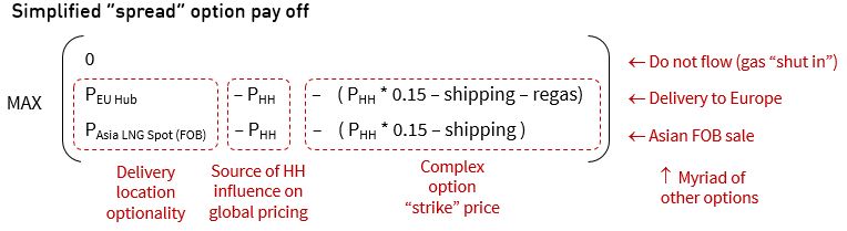
Gas vs coal switching in Europe: numerical analysis

Posted on June 6, 2016January 16, 2020 by David Duncan

Over the 2016-19 period, LNG liquefaction capacity under construction is set to increase global LNG supply by approximately 150 bcma. Current rates of global LNG demand growth are not high enough to absorb this swell in new supply.

Europe will play a key role in balancing the global gas market, given the status of liquid European hubs as the ‘market of last resort’ for surplus LNG. In turn the impact of LNG flowing into Europe will be one of the key factors driving the evolution of European hub pricing dynamics.

The switching of gas-fired power plants for coal plants is set to be the frontline mechanism that enables Europe to absorb more gas. But what incremental volumes of gas can the power sector burn, and how do these volumes change with market prices?

In last week’s article we set out and ranked the key power markets that drive the switching of gas for coal fired power plants in Europe. We also showed an illustration of the gas vs coal price boundaries which provide a benchmark for the market conditions required for switching.

In today’s article we transition from a comparison of individual power markets to look at an aggregate pan-European view. We do this in order to quantify the aggregate European switching volume potential and its relationship to relative gas vs coal prices.

Putting numbers around the switching problem

It is difficult to perform a robust estimate of aggregate gas vs coal switching potential in Europe without modelling the underlying dynamics of the individual power markets which drive switching. To enable this, we have set up a scenario in our pan-European power market model that reflects current forward market pricing for fuels. This provides a benchmark for aggregate power sector gas demand given current gas and coal market prices.

In order to analyse aggregate gas vs coal switching potential, we then run multiple combinations of gas and coal prices through the pan-European power market model. This allows us to produce gas switching demand curves for the different combinations of market prices shown in the left hand panel of Chart 1.

Chart 1: Aggregate European gas switching volumes vs market prices

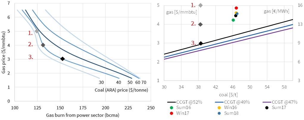
Source: Timera Energy

Each line in the left hand chart can be thought of as an aggregate gas demand curve for the European power sector. In other words the lines show aggregate gas burn (bcma) as a function of gas price. Five different demand curves are shown for different coal prices.

The central (darkest blue line) shows switching dynamics at current forward coal prices for European delivery (approximately 50 $/t). As you move from left to right down this line, gas switching volume increases as gas prices fall.

We have then also produced demand curves for incremental changes of 10 $/t in coal prices away from the 50 $/t anchor case (shown as the other blue lines on the left hand panel). It is interesting to compare the shape of these demand curves at different levels of coal prices:

Coal price 70 $/t: This switching line illustrates a scenario where coal prices rise around 20 $/t higher than current market levels. In this situation there is an almost linear relationship between gas prices and aggregate European gas switching volumes. This is because with significantly higher coal prices, gas-fired plants across Europe are broadly on equal competitive terms versus coal plants, with load factors and gas burn increasing steadily as gas prices decline.
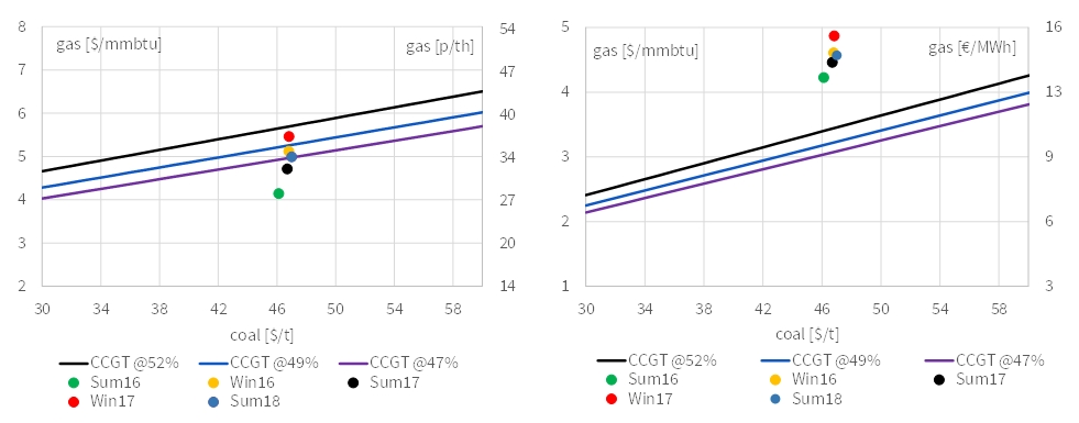
Coal price 40 $/t: This switching line shows a scenario where coal prices fall relative to gas prices, inducing a pronounced boomerang shape in the switching line. This shape relates to differences in capacity mix across European power markets. Some substitution of gas for coal plants occurs at higher gas prices (e.g. 5-6 $/mmbtu) in markets where CCGTs play a more dominant role in the capacity mix (e.g. UK and Italy). But in a price range below this (4-5 $/mmbtu), the rate of gas switching declines as gas prices fall, before increasing again at lower gas prices (e.g. 3-4 $/mmbtu). This is because larger gas price declines are required to trigger material switching in the Continental power markets which are currently dominated by coal generation (e.g. DE, NL). This can be seen via the Netherlands switching boundary chart in the right hand panel (which we showed last week), where gas prices need to fall towards 3 $/mmbtu to induce baseload switching of CCGTs for coal plants.

The demand curves shown in Chart 1 enable a more practical analysis of potential switching volumes in Europe given different combinations of gas and coal prices.

Switching volume response to absorb oversupply

In order to draw some conclusions on aggregate European switching volume potential it is helpful to consider two cases:

An isolated gas price decline: This provides a useful upper bound for switching potential e.g. in a scenario where gas prices weaken as oversupply grows, but other commodity prices (e.g. coal and oil) stabilise around current levels.
A correlated gas and coal price decline: This provides a more conservative estimate of switching potential assuming gas and coal prices decline together, but with gas prices falling at a faster rate than coal (as has been experienced so far in 2016).

European hub prices could fall another 1.00-1.50 $/mmbtu before truly converging with Henry Hub (as we set out here). If this occurred as an isolated decline in gas prices from current levels (a little above 4 $/mmbtu) it could generate an estimated 30-40 bcma of gas switching volumes.

If on the other hand coal prices declined in tandem with the 1.00-1.50 $/mmbtu fall in gas prices, for example to 40 $/t, then we estimate it could generate gas switching volumes of 15-25 bcma This is likely to be more like 0-10 bcma in the case of a more substantial decline in coal prices to 30 $/t.

Switching dynamics are a big deal for the European gas market. Switching volume behaviour is set to play a pivotal role in balancing the European gas market over the remainder of this decade. But European power sector switching is also a major concern for the global gas market.

The extent to which the European power sector can absorb surplus LNG may also be a key driver of US exports volumes and flows. If the growth in global oversupply exhausts the switching potential in Europe, the role of market of last resort will need to transition to North America. This would mean that US export shut-ins would be required to absorb additional surplus LNG.

Article written by David Stokes & Olly Spinks

Gas vs coal switching in Europe: key markets

Posted on May 30, 2016January 16, 2020 by David Duncan

The displacement of coal plant by gas plant is one of the key current focus issues in the European energy industry. A sharp decline in coal prices from 2010 to 2014 drove much of Europe’s gas fired capacity out of merit. But gas plants have started to make a comeback in 2016. Falling gas hub prices are favouring CCGTs over coal plants and some of the coal for gas switching from earlier this decade is beginning to reverse.

Gas vs coal switching is an issue that spans gas and power markets in Europe. Switching is an important driver of power prices, load factors and generation margins in power markets. But it also determines the level of incremental gas demand from the power sector as hub prices decline. In other words it is the primary driver of the shape of the demand curve for the European gas market. As such, it is also important in a global LNG market context given switching is playing an important role in stemming the decline in NBP/TTF gas prices towards Henry Hub.

While the role of switching is being widely debated across the industry, there is less clarity around the practical impact of switching on volumes and prices. So we are publishing a numerical analysis of European gas vs coal switching potential in a two article series. This week we address the dynamics that drive switching and set out the key power markets involved. Then next week we analyse aggregate switching volumes across Europe, given different levels of gas and coal prices.

The drivers of power sector switching

There are several important factors that determine the contribution of individual power markets to Europe’s aggregate switching potential:

Market size: The scale of generation output in the market is clearly a defining factor. This means a focus on the larger power markets in Western Europe.

Gas capacity: The volume of installed gas-fired generation capacity is one factor determining potential gas burn.

Coal capacity: The other side of the switching equation is determined by the volume of installed coal capacity which impacts the degree to which substitution is possible.

Gas plant responsiveness: The existence of significant volumes of gas and coal capacity does not on its own determine switching potential. The role of gas plant in the merit order and the responsiveness of gas burn to changes in fuel prices is an important overlay. Other considerations such as the range of gas plant efficiency and volumes of must run renewable & CHP output also need to be accounted for.

The ability of gas plant to respond to market price changes is the most important dynamic impacting current switching dynamics. This is best illustrated via two practical examples.

Chart 1 shows a current overview of the gas vs coal switching boundaries in the UK and Netherlands power markets.

Chart 1: UK vs NL coal vs CCGT switching boundaries

Source: Timera Energy

These charts show whether current forward market prices favour gas or coal burn. The coloured dots represent different combinations of gas and coal prices for seasonal forward contracts over the next two years. The diagonal lines show the baseload switching boundaries for CCGT plants of different efficiencies (a 52% new plant through to a 47% 1990s plant). In simple terms, if the dots sit below the diagonal switching lines then market prices favour gas burn. If the dots sit above the switching boundaries they favour coal burn.

The UK and Netherlands both have significant volumes of gas and coal capacity installed. But the role and responsiveness of gas plant is very different across the two markets:

In the UK: Gas fired plants dominate the setting of marginal wholesale power prices. CCGTs also benefit from the UK carbon price floor which disadvantages coal plants. This means there is already significant switching taking place at current gas price levels, with newer CCGT running baseload and older CCGT running mid-merit, displacing the majority of coal plant capacity from the merit order.

In the Netherlands: Gas fired plants dominate the capacity mix like in the UK. But a significant portion of this gas capacity is must run CHP plant which is not responsive to market prices. In contrast to the UK, power prices are predominantly set by cheaper coal fired capacity in neighbouring Germany. This means that gas vs coal switching plays a limited role at current market prices (with the dots sitting 2-3 €/MWh above the switching boundary in the NL chart).

Key switching markets in Europe

The next step is to translate these drivers into a practical ranking of switching potential across European power markets. This is where the problem can be narrowed down to several key markets. More than 70% of European switching potential is focused on these top 5 markets:

UK
Italy
Spain
Germany
Netherlands

If you also include the next 5 most important markets (Turkey, France, Belgium, Austria, Portugal), it accounts for approximately 90% of European switching potential. Turkey comes in a close 6th after the Netherlands, with higher installed capacity but some constraints around switching responsiveness.

In Chart 2 we show a representation of switching potential by market that combines some of the drivers listed above. The chart shows installed capacities of gas and coal plant on the vertical and horizontal axes respectively. The size of the bubbles for each market represents the historical range of gas burn in the market over the first five years of this decade (2010-14). This captures the transition from coal vs gas competitiveness being relatively balanced (2010-11) to strongly coal favouring (2013-14).

Chart 2: European gas vs coal switching benchmarks by market

Source: Timera Energy

The advantage of this historical measure is that it is a transparent empirical benchmark. The disadvantage is that it is backward looking. While gas vs coal switching is the main driver of gas burn changes, there are some other factors in play (such as renewable erosion of gas plant load factors). As a result this measure provides an upper bound for switching potential.

When we come back in our second article next week we use an alternative forward looking approach to quantify gas switching volume potential. We use our pan-European power model to analyse gas switching volumes given different combinations of gas and power prices.

This approach illustrates the drivers set out this article, but provides a more detailed view of how switching is likely to impact gas and power markets over the next 3 years. Historical switching may be starting to reverse. But the market dynamics in the second half of this decade are going to be very different to the first.

Article written by David Stokes & Olly Spinks

Long term contract pricing: 5 key drivers

Posted on May 23, 2016January 16, 2020 by David Duncan

Long term contracts play an important role in enabling the owners of flexible gas and power assets to monetise asset value and manage market risk. Common examples in power markets include tolling contracts, power purchase agreements and fuel supply agreements. Just as common in gas markets are capacity contracts on gas storage facilities, pipelines and regas terminals.

Long term contract (LTC) pricing is often a key driver of an asset investment case. The negotiation of contract pricing terms can be pivotal in getting past the Financial Investment Decision (FID) hurdle or raising debt financing for new assets. Long term contract pricing also typically plays an important role in determining bid price levels and financing terms for transactions involving existing assets.

While the importance of LTCs is clear, they present a key challenge. It is difficult to come by transparent benchmarks for LTC pricing. Pricing terms are usually closely guarded commercial secrets and the unique terms of specific contracts make it difficult to compare prices across contracts.

In this article we recognise these constraints, but focus on a structured way to understand & quantify drivers of LTC prices. This article follows on from two previous articles in a series we are publishing on LTCs:

5 key drivers of LTC pricing

The first thing that is important to recognise is that forward markets drive LTC value. This is the case even if the duration of the LTC extends well beyond the forward market horizon.

Growing liquidity in European gas and power markets means that the pricing of LTCs is underpinned by the prevailing forward price dynamics against which LTC value can be monetised. This is reinforced by the fact that LTC pricing is increasingly being influenced by trading focused intermediaries e.g. commodity traders, banks or other energy trading desks. These players may not have a specific portfolio requirement for LTC flexibility, but are prepared to price and monetise LTC value using underlying commodity markets.

To put some structure around how LTC prices relate to underlying market dynamics it is useful to deconstruct price drivers into five key categories set out below.

Exposure: The structure of LTC pricing terms in relation to underlying commodity prices (e.g. fixed price, price indexation, upside sharing or cap & floor terms).
Intrinsic value: The degree to which LTC value can be hedged against current forward market prices (i.e. the ‘in the moneyness’ of the contract).
Market conditions: The prevailing market pricing of flexibility contained in the LTC (e.g. driven by liquidity, price volatility, pricing/availability of alternative forms of flexibility).
Duration: The term of the contract which influences available liquidity to manage LTC exposures as well as the level of uncertainty over future price evolution.
Portfolio drivers: Other portfolio related value driven by factors such as ‘insurance premia’, risk limits, security of supply mandates or strategic considerations.

Chart 1, illustrates how these 5 key drivers relate to asset margin distributions.

Chart 1: Asset margin and the 5 key drivers of LTC pricing

Source: Timera Energy

The influence of these 5 drivers can vary significantly by contract, underlying asset and market. For example:

UK interconnector: the pricing of fixed price UK electricity interconnector contracts is strongly influenced by relatively high intrinsic value given the prevailing forward market premium of UK over Continental power prices (i.e. LTC pricing is driven by the fact that interconnectors are deep ‘in the money’).

German fast cycle storage: long term contracts on fast cycle gas storage capacity have very little intrinsic value but are strongly influenced by market conditions e.g. the level of prompt gas price volatility and the pricing of alternative sources of gas deliverability.

Southern European pipeline capacity: The value of LTCs on gas pipeline capacity into Italy or Spain can be strongly influenced by strategic portfolio considerations. Non incumbent players may pay a premium for external access to liquid European hubs, given cross border capacity availability constraints.

To illustrate how the five LTC pricing drivers interact, we return the UK CCGT tolling contract example we set out in our first article in this series.

A UK tolling contract case study

This case study has a current relevance given that a number of CCGT project developers are trying to structure tolling contracts to support the bidding of CCGT development projects into this year’s UK capacity auction.

Exposure:

The structure of LTC pricing terms determine contract exposures to underlying commodity prices. Tolling contracts are typically structured on a fixed price annual capacity fee basis (i.e. £/kW/yr). This acts to transfer market risk from the power station owner to the tolling counterparty. But tolling contracts can also contain indexation, upside sharing or availability risk sharing terms that mean that the owner retains a portion of market risk.

Intrinsic value:

CCGT intrinsic value is a rapidly evolving concept in the UK power market. CCGTs have increasingly come back into merit in 2016 as gas hub prices have declined. This supports the value of longer term tolling contracts, which have been difficult to source over the last 5 years as load factors have declined. However forward clean spark spreads remain relatively weak which has a strong influence on the way that tolling contracts are priced.

Market conditions:

Aside from spark spread levels there are several other market related factors that impact tolling contract prices. A significant portion of UK CCGT value is realised in the prompt horizon as power price granularity increases. Power price volatility on the other hand has been relatively low which reduces the value of CCGT flexibility. The depth of buyer interest has also been limited given negative sentiment on CCGT value and the fact that utilities (arguably the natural buyers of tolling contracts) are encumbered with write-downs on their own CCGT assets.

Duration:

The term of UK tolling contracts is a key factor driving pricing. A number of counterparties are prepared to price 3 to 5 year tolling contracts given an ability to hedge a significant portion of forward exposures (with UK power market liquidity reasonable out for 3 to 4 seasons). But a 7-10 year tolling contract to support financing of a new CCGT project may be priced at a substantial haircut to reflect a lack of forward liquidity over this horizon and considerable market uncertainty in the 2020s.

Portfolio drivers:

Portfolio drivers have not had a strong influence on UK CCGT tolling contract value. This could be different if UK utilities had a requirement for gas-fired flexibility to hedge their supply portfolios. But existing flexibility from vertical integration has neutralised this impact. Pricing is instead firmly focused on the expected value of tolling contracts that can be monetised against underlying power, gas and carbon markets.

So now we’ve considered 5 key drivers of LTC prices and a case study, how do we approach putting a number on LTC price levels?

5 key drivers of LTC price quantification

The most sensible way to approach LTC price quantification is to use a similar approach to the trading desk counterparties that typically set LTC price levels. The techniques used to value LTCs are becoming more standardised across trading desks from utilities, commodity traders or banks. These again lend themselves to deconstruction into 5 key drivers:

1. Intrinsic value: LTC value that can currently be hedged against forward curves typically defines an important lower bound for LTC price level. It is transparent and relatively easy to calculate.

2. Full merchant value: The most important benchmark determining LTC price levels is the expected merchant value that can be generated via the contract. On top of intrinsic value that can be locked in today, this consists of:

value beyond the liquid forward curve horizon
shape value as forward contracts become more granular closer to delivery, allowing additional flexibility value to be monetised
value from using LTC flexibility to respond to shorter term price volatility (often termed extrinsic value)

Quantifying expected merchant value is typically done using complex models that capture the interaction between (1) commodity price uncertainty and (2) asset / contract flexibility and constraints. However, model complexity comes a with a health warning. Robust parameter estimation, sensible treatment of practical value monetisation issues and experienced judgment in interpreting model results are a prerequisite for effective modelling.

3. LTC haircut: A counterparty bidding for an LTC will not pay its expected merchant value. Instead the counterparty will discount expected value to reflect its costs of monetising LTC value. The most important costs are associated with risk capital (to back potential swings in LTC value) and market transactions costs (e.g. bid/offer spreads & credit costs). These costs can be quantified and compared with empirical benchmarks to estimate LTC haircuts.

4. Historical value: Estimating LTC value based on historical market conditions provides a clean and transparent measure to benchmark modelled expected merchant value.

5. Transaction implied value: There are often interesting LTC value benchmarks that can be implied from relevant asset transactions or other LTC prices. These can provide very useful information on market conditions (e.g. expectations on volatility or existence of any portfolio driven value).

Narrowing in on pricing bounds

Using these approaches to bound LTC price quantification provides a much greater insight than a simple scenario based approach. It also acts to build confidence around upper and lower pricing bounds and key pricing inflection points.

Ultimately the price of a specific LTC will come down to a unique set of circumstances. But having a structured framework for understanding and quantifying the drivers of LTC pricing can make life much easier.

Article written by David Stokes & Olly Spinks

US exports and the trans-Atlantic cost question

Posted on May 16, 2016January 16, 2020 by David Duncan

The costs of moving LNG from the US to Europe was one of the key focus points at last week’s Flame conference. A number of divergent views were presented on the level of costs that US exporters need to recover in order to send LNG to Europe. However there was a consensus that the trans-Atlantic cost differential was likely to become a key factor driving gas flows and hub pricing dynamics.

Timera Energy gave two presentations at Flame that set out our view on trans-Atlantic variable costs and the influence of these in driving US vs European hub price differentials. Given the interest this topic attracted, we have focused today’s article on setting out a more detailed breakdown of our assumptions, with a particular focus on the treatment of shipping costs.

US export contract dynamics

US export contracts are structurally different from other LNG contracts. They are structured as a liquefaction capacity option rather than a conventional gas supply agreement. This means contracts have the inherent flexibility to:

Send export volumes to the highest priced market (on a spot price netback basis)
Ramp down contract volume take to zero if market prices do not cover variable costs

Contract holders pay a fixed capacity fee (e.g. 2.25 $/mmbtu for Sabine Pass). But importantly this is a sunk cost and has no bearing on flow decisions which are driven by variable costs. This means that US export contracts are essentially a complex option on the spread between Henry Hub and regional spot LNG prices. We show a simplified representation of the payoff for this option in the diagram below.

Diagram 1: US export spread option payoff function

Source: Timera Energy

The strike price of this option is driven by the variable costs of (i) liquefaction (ii) shipping and (iii) regas as we set out in last week’s article. We also defined our estimate of a current trans-Atlantic variable cost range for delivery of US exports to Europe as follows:

Upper bound: 1.10 $/mmbtu
Lower bound: 0.60 $/mmbtu

It is important to note that these numbers are defined using current market fuel and charter rates which may change going forward.

US export volumes are likely to continue to flow to Europe as long as the spread between NBP/TTF and Henry Hub prices exceeds the upper bound of trans-Atlantic variable costs. Exports may of course flow elsewhere (e.g. to Asia or South America) if netback prices are more attractive.

If trans-Atlantic price spreads fall below the upper bound then a portion of US export volumes may be ‘shut in’. If price spreads fall below the lower bound it is likely that all US export volumes will be shut in. However the cost cut off point for export volumes will vary based on contract, terminal and counterparty specific factors. One of the most important drivers will be the treatment of shipping costs.

Recap on shipping cost components

The key components that make up the cost of shipping LNG are as follows:

Chartering fee: This is the payment for securing access to shipping capacity by chartering a vessel. There are broadly three ways to secure access to shipping capacity: (1) own vessel capacity (2) long term time charter and (3) spot (short term) time charter (e.g. for a single voyage). We tend to focus on spot charter rates as the benchmark driving marginal shipping costs.

Brokerage: Vessel charters are typically arranged through specialist brokers and attract a 1-2% fee.

Fuel consumption: The voyage fuel or ‘bunker’ consumption is directly proportional to the distance and speed of the vessel. This is typically the second largest cost component after the chartering cost. The added complication for LNG vessels is the different propulsion mechanisms and fuel burn options. Most LNG vessels can burn fuel oil, boil-off gas or a blend of both in their boilers. As a result the calculation of fuel cost is closely tied to that of boil-off gas. Natural boil-off occurs at a rate of approximately 0.15% of inventory per day and at times boil off is forced above this level to further reduce the fuel oil requirements. Some modern LNG vessels also have the ability to re-liquefy boil-off gas, keeping the cargo whole (and allowing the use of more efficient diesel engines). Calculation of the direct fuel consumption is fairly straightforward but the opportunity cost of LNG boil-off is also an important consideration.

Port costs: The components and level of the costs of loading and unloading at ports can vary widely depending on location. For example, ports in less stable regions can levy large security charges associated with ensuring the safety of the vessel.

Canal costs: Transit costs have to be paid for using the cross-continental Suez and Panama canals. Suez canal transit costs are a complex function of vessel dimensions and cargo (laden voyages being more expensive) and LNG vessels are entitled to a 35% discount after which the costs are in the region of USD 300-500k per transit. With the Panama canal widening project, around 80% of LNG vessels are able to make the transit. This reduces the distance from 16,000 to 9,000 miles from the US gulf coast to premium Asian markets.

Insurance costs: Insurance is required for the vessel, cargo and to cover demurrage (liabilities for cargo loading and discharge overruns).

Breaking down trans-Atlantic costs

Chart 1 sets out the component breakdown of our upper and lower bound estimates for trans-Atlantic costs.

Chart 1: Current Gulf Coast to UK shipping cost bounds

Source: Timera Energy

The basic shipping cost calculations assume:

160 MT vessel
Journey distance 4,900 NM
Travelling at 14 knots running on boil-off (some small FO in-port consumption)
25k pd charter rate
Plus allowances for port and other costs
Covers round trip journey (laden and unladen voyages)

Our upper bound assumes full fixed and variable cost recovery and the lower bound assumes exclusion of sunk charter costs and regas costs (although in reality a small proportion of the regas costs are likely to be variable).

There are some important factors which can influence these cost estimates. Fuel costs will vary by vessel type, with a key consideration being to what extent the vessel runs on conventional marine fuel (e.g. gas oil or fuel oil) versus boil-off. Some vessels can make the trans-Atlantic journey entirely via use of boil-off albeit at a reduced speed (14 knots vs 19 knots). Chart 2 illustrates the impact of running on boil-off vs fuel oil for a Gulf Coast to UK journey.

Chart 2: Impact of propulsion methods on shipping costs

Source: Timera Energy

Running on fuel oil reduces journey time by around 4 days (or 8 days for a return journey) when compared to running on boil-off. The reduction in charter rates from the quicker journey combined against the incremental FO costs can be compared to a longer journey but practically no fuel costs when running on boil-off. Current voyage economics suggest that running on boil-off is the lower cost option. We have assumed 100% boil-off operation in our estimates above, but these increase if vessels burn conventional fuels.

Another key point is the treatment of fixed and variable costs of the ballast (unladen return) voyage. When shipping margins are healthy it is reasonable to assume that in some cases that ballast voyage costs can be internalised by the shipping operator. But under current conditions, low charter rates do not support annual vessel cash costs, so it is reasonable to assume that the variable cost of the ballast journey is included in costs calculations. These are quite low if the vessel is assumed to run on boil-off.
We have not included an allowance for port costs in the US liquefaction fee. There is a lack of transparency as to what charges will be levied on LNG carriers but for other vessel types in can be upwards of $500k.

US cargoes will go to the highest bidder

Any differences in the cost of getting gas liquefied and loaded onto a vessel are likely to be important in determining the ‘merit order’ of US export volume shut ins. But in our view the shipping and regas costs of the holders of US export contracts will not necessarily drive trans-Atlantic flow dynamics. US cargoes will likely be sold to intermediaries if they have access to lower shipping and regas costs.

This is where we believe that NBP/TTF vs Henry Hub shut in spread levels may surprise on the downside. In other words shut ins may be driven more by the lower bound (reflecting sunk shipping and regas costs) than the upper bound (reflecting full variable cost recovery). Cargos will go to the highest bidder and that is likely to be the party with the lowest variable cost structure. Don’t underestimate the ability of market driven innovation to erode the trans-Atlantic price spread.

Article written by David Stokes and Olly Spinks

What does Henry Hub convergence mean?

Posted on May 9, 2016January 16, 2020 by David Duncan

Prices at the UK NBP and US Henry Hub converged completely during the last global supply glut in 2009-10. This was a simple consequence of global oversupply. The sale of surplus LNG into the European gas market drove down hub prices to the point that it was more profitable to divert LNG to the US.

Stepping forward to the current phase of oversupply could this happen all over again? The answer to this question is not a simple yes or no. Convergence is definitely possible as new LNG supply ramps up over the next 2 to 3 years (as we set out here). But the introduction of US exports means that it is likely to be a different sort of convergence to that experienced in 2009-10.

Variable costs of moving gas across the Atlantic is key

In a world of US exports, the variable cost of moving LNG from the US to Europe plays an important role. It is this cost that is the key driver of the trans-Atlantic price differential. The trans-Atlantic variable cost can be split into three components as illustrated in Chart 1:

Liquefaction: the cost of getting gas liquefied and onto a vessel at a US terminal
Shipping: the cost of transporting gas to a NW European regas terminal
Regas: the cost of getting gas to the European hub

Chart 1: Benchmarks for trans-Atlantic variable cost

The liquefaction cost is relatively straightforward as it is specified in most US export contracts at 115% of gas cost (~0.30 $/mmbtu with Henry Hub at 2 $/mmbtu). In some cases there may also be some incremental transport cost for getting gas to the terminal.

The shipping cost is the most complex component and varies by company. First, the physical vessel characteristics (size and technology) has an important influence on costs. Second, some cost elements are truly variable (e.g. propulsion), but other elements may have sunk cost characteristics (e.g. some of the charter cost components). Third, allocation of the costs of ballast or return voyages is not straightforward. Finally, propulsion costs can be substantially reduced for longer voyages by running vessels at lower speeds on LNG boil off (e.g. 14 knots vs. 19 knots on fuel oil). We will be revisiting the complexities of shipping cost calculation dynamics in an up coming article.

If the trans-Atlantic price differential really tightens, then cargoes will likely be flowed by players with access to the cheapest transport. This may mean US export contact holders selling cargoes to third parties with lower transport cost dynamics. This means the true variable cost of trans-Atlantic transport (excluding sunk costs) is likely to be the most important benchmark providing support for NBP vs HH price spreads.

Regas terminal costs can also have sunk cost characteristics. This is because many shippers have access to existing contracted terminal capacity in Europe. It is typically regas costs in the North West European terminals (0.2-0.5 $/mmbtu) that are relevant given that:

costs are lower in the UK and Benelux (e.g. higher than 1.50 $/mmbtu in Italy) and
terminals offer easier access to liquid hubs (NBP and TTF).

Chart 1 illustrates an upper and lower bound for trans-Atlantic LNG costs. A lower cost bound of about 0.6 $/mmbtu comes from assuming all charter and regas costs are sunk and the maximum benefit is gained using boil-off to reduce fuel costs. This can be contrasted with an upper bound of around 1.15 $/mmbtu if all variable cost elements are included.

Impact of trans-Atlantic cost on hub prices

Spot prices at North West European hubs are currently around the 4.10 $/mmbtu level. Spot US gas prices at Henry Hub (HH) are close to 2.10 $/mmbtu. This 2.00 $/mmbtu NBP vs HH differential is relatively stable across the forward curve horizon as shown in Chart 2.

Chart 2: NBP vs Henry Hub price differential and arbitrage range

As oversupply in the global LNG market increases over the next two years, this US vs European price differential may narrow. But in a world of US exports the variable cost of trans-Atlantic arbitrage becomes a powerful force working to maintain a positive trans-Atlantic price spread.

35 bcma of US export capacity is due to come online by the end of 2018. This is set to swell to around 80 bcma by the end of the decade. US exports of this scale provide an important support mechanism for both global gas prices and the trans-Atlantic price spread.

If NBP vs HH price differentials fall below the variable cost of moving gas from US to European hubs, then US exports will be ‘shut in’. This acts to support trans-Atlantic price differentials in two ways. Firstly it reduces global LNG supply, supporting European hub prices. Secondly the shut in of US gas increases supply at Henry Hub, putting pressure on US gas prices.

As US exports ramp up, the factors described above will act to increase the influence of Henry Hub on European hub prices. It will also strengthen the Atlantic Basin price signal as the main driver of global LNG pricing. This means it is important to start to look to the east. Henry Hub prices are going to feature more strongly in European gas portfolio exposures, whether explicitly or implicitly. And this is an important consideration for portfolio management and development.

Article written by Olly Spinks & David Stokes

Timera Energy is presenting at Flame this week.

Olly Spinks is speaking today on the impact of US exports on European hub prices. David Stokes is speaking on Tuesday on European hub price dynamics and gas portfolio exposures.

Anatomy of a spring short squeeze

Posted on May 2, 2016January 16, 2020 by David Duncan

Last week saw some extreme swings in European gas hub prices. The combination of an early spring cold snap and North Sea supply outages caused the NBP forward curve to explode 20% higher than levels seen the previous week. This move was mirrored across Continental hubs led by the Dutch TTF. But the action was not all one way, with prices plunging 10% in a day last Thursday. Price volatility has returned to European hubs despite the weight of oversupply.

The impact of short term supply and demand shocks such as those last week is typically focused in the front of the forward curve e.g. via surging day-ahead and within-month prices. But last week’s moves saw large parallel shifts in prices across the forward curve. That is a characteristic of a classic short squeeze in a market that has been weighed down by strong bearish sentiment since the start of the year.

Prompt wags the tail

To illustrate these recent price moves, Chart 1 shows NBP forward curves (based on ICE futures contracts) from three days over the last two weeks:

Bottom curve (black): NBP forward curve from the beginning of the previous week (18^th Apr)
Top curve (dark blue): curve from last Wednesday’s close (27^Th Apr), approximately 20% higher
Middle curve (light blue): curve from last Thursday (28^th Apr), showing a 10% fall in the front of the curve.

Chart 1: NBP forward curve moves over the last two weeks

Source: Timera Energy (ICE data)

Last week’s price surge that culminated on Wednesday was fuelled by unseasonably cold weather in North West Europe. This coincided with production outages on the Norwegian Continental Shelf and an outage at the Easington terminal in the UK.

All of these factors are relatively short term in nature. But the chart illustrates a parallel move higher in prices across the forward curve. The transmission mechanism from prompt prices to the front of the curve relates to gas storage dynamics. Last week saw a sharp increase in storage withdrawals to plug the supply gap, in a period where seasonal storage facilities are typically injecting gas in preparation for next winter. Pulling gas out of store means greater volumes need to be purchased for injection across the summer, triggering a rally in summer hub prices. But this is only part of the story. Portfolio positioning is likely to have played a more significant role in the price swings than any fundamental factors.

Short squeeze dynamics

European hub prices have been weighed down since the start of 2016 by lower oil prices, robust production volumes and rising LNG imports. Gas market sentiment (e.g. as measured by Bloomberg) has been consistently bearish. And it is easy to see why against the fundamental backdrop we set out last week. But bearish fundamentals over a two year horizon do not preclude sharp moves higher in the shorter term.

One of the practical implications of strong bearish sentiment is that gas portfolios tend to be positioned for further price declines. This may be via trading desks being outright short gas. Or it may relate to portfolio’s being underweight hedge volumes required to meet demand. Either way it leaves the market exposed to sudden shocks to the upside.

Last week’s move higher in gas prices also occurred against a backdrop of a similarly unexpected rally in oil prices since the start of April. The combined gas and oil rally is likely to have been partially fuelled by energy trading desks being forced to buy volumes as portfolio risk management limits are breeched (e.g. ‘stop loss’ and ‘VaR’ limits). This can create a self-reinforced surge as the price rally triggers further stop loss buying.

These are the classic characteristics of a short squeeze. And this logic is reinforced by the rapid decline in European hub curves that followed last Wednesday’s surge. Stop loss buying is often a short lived phenomenon with prices spiking but leaving a vacuum below. When the self-reinforced buying frenzy subsides, fundamental market drivers reassert themselves.

Price moves relative to other benchmarks

Last week’s price moves illustrate some interesting dynamics with respect to Europe’s role in driving global LNG spot prices. The rally in North West European hub prices over the last two weeks has supported a recovery in Asian spot LNG prices. This has coincided with a re-emergence of short term buying interest from Japan, Taiwan and Argentina, but NBP is the key benchmark pulling cargo prices higher.

Last Wednesday’s European price surge saw the unusual phenomena of NBP temporarily trading at a premium to spot LNG prices in Asia and South America. The front month NBP contract closed at 4.70 $/mmbtu on Wednesday, a premium of 0.25 $/mmbtu over spot LNG benchmarks around 4.45 $/mmbtu (as shown on Chart 1). Chart 1 shows how this premium was short lived, with Thursday’s fall reinstating the usual transport cost driven discount of NBP to spot LNG prices.

Last week’s price behaviour illustrates some of the relative pricing dynamics we set out in our last article. The impact of the short squeeze in driving European forward prices higher quickly ran out of steam given strong overhead price resistance from:

LNG spot prices, reflecting the current global surplus of flexible LNG
Oil-indexed contract prices, reflecting additional volumes of pipeline gas that can flow into hubs at higher prices

These factors weigh against the chances of a structural recovery in hub prices across the rest of 2016. But the events of the last week have breathed some life back into European gas price volatility. This is a key price signal for the battered value of gas supply flexibility. As 2016 evolves it will be interesting to see if the recovery in volatility is temporary in nature or the start of something more enduring.

Article written by David Stokes & Olly Spinks.

European gas market: current supply & demand balance

Posted on April 25, 2016January 16, 2020 by David Duncan

The next two years are set to be an important period of transition for the European gas market. LNG imports are increasing as Europe adapts to its role as the global gas sink. In addition, oversupply at European hubs is eroding the traditional price setting role of oil-indexed Russian gas contracts. But as 2016 progresses and hub prices fall, there is clear evidence of evolving demand response from the power sector.

The European gas market is underpinned by a complex network of interconnected hubs, delivery routes and contractual obligations. In our view this undermines the effectiveness of traditional ‘field, flow & flange’ analysis to gain any sensible view of how market drivers interact to determine price dynamics.

A more practical approach is to focus analysis on the interaction between demand and the key tranches of flexible supply that set hub prices (e.g. Russian swing, flexible LNG and Norwegian production flex). We have previously set out how we do this using our analytical framework for European gas market analysis.

This approach has helped us to anticipate some of the major inflection points in European gas pricing over the last three years. For example the Summer 2014 price slump that marked the start of the current phase of oversupply and the ‘tipping point’ decline currently in progress as European prices fall towards Henry Hub support.

In today’s article we revisit this framework to set out our current view of the supply and demand balance in the European gas market. We also highlight a number of factors to watch in order to determine the evolution of market dynamics going forward.

European supply and demand balance: an annual view

There are two important considerations that can greatly simplify European hub price dynamics:

Grouping sources of supply with similar pricing and flow dynamics
Focusing on the flexible volumes of gas that drive hub pricing at the margin

The first of these tasks is helped by the fact that most sources of European supply are under long term contracts that use a similar structure. The second task is assisted by the fact that only a relatively small volume of total European supply actually has the flexibility to respond to changes in market price.

Chart 1 illustrates the current European supply and demand balance using this approach. It is important to note that the chart summarises supply and demand at an annual level. We come back below to some of the important within-year drivers of pricing and flows.

Chart 1: 2016 annual European supply and demand balance

Source: Timera Energy

Supply

The chart shows sources of European gas supply grouped into several key tranches:

Inflexible price taking supply: consisting of (i) pipeline contract ‘take or pay’ volumes (ii) inflexible LNG contract volumes and (iii) domestic production (very low variable cost ). These ‘price taker’ volumes flow regardless of hub price levels.
Norwegian flexible volumes: consisting of Norwegian production flexibility and flexible hub indexed contract volumes. These volumes are also effectively ‘price taking’ given Norway produces to an annual production target, but they are shown at a slight discount to current hub prices to reflect the fact that flows are optimised against hub prices.
Flexible LNG volumes: made up of divertible European LNG supply contract volumes and LNG spot cargoes surplus to the requirement of other regions. Volume and flow depends on netback LNG spot price differentials relative to European hub prices.
Pipeline contract flexibility: from predominantly Russian oil-indexed swing contract volumes above ‘take or pay’ levels.
Spot Russian & incremental LNG: gas volumes that may be induced to flow into European hubs if prices rise sufficiently to attract (i) incremental Russian spot flows and (ii) diversion of LNG from other regions (predominantly Asia where fuel substitution is possible, typically to oil products).

The interaction between tranches 2, 3 and 4 and demand is the place to focus in order to understand price dynamics.

Demand

European gas demand is relatively price unresponsive in the shorter term, except for the power sector. The downward slope of the demand curve in the chart reflects the potential impact of coal to gas plant switching across European power markets as gas prices fall.

The amount of additional gas demand that is generated at lower hub prices depends on relative gas vs coal pricing. But there is 50+ bcm of switching potential if coal prices remain relatively stable while gas hub prices continue to decline towards Henry Hub. We will come back in a subsequent article to explore this dynamic in more detail, but it is going to be a key factor driving gas market dynamics over the next 2-3 years.

Pricing at the margin

Declining hub prices in 2016 are being driven by a battle to place Norwegian flex, LNG imports and Russian pipeline volumes across European hubs. This is in addition to the large volume of ‘must flow’ gas shown at zero price in the chart.

Oil-indexed contracts have historically played an important role in setting hub prices at the margin (the intersection of supply and demand). Oil-indexed prices tend to act as a magnetic force given the use of swing gas to balance the market. But as 2016 progresses into 2017, the impact of the tipping point we foreshadowed this time last year looks set to gather momentum.

A combination of robust production flows (particularly from Norway) and rising LNG imports are pushing oil-indexed contract prices off the margin. The result is that hub prices (currently around 4.00 $/mmbtu) are falling below oil-indexed contract benchmarks (4.50+ $/mmbtu). With hub prices at a discount to contract prices, suppliers are incentivised to reduce contract volumes to take or pay levels.

The damage to hub prices is being caused by increasing volumes of supply being pushed in to the European market to left of the margin. Robust production levels and rising LNG imports are forcing the supply curve down the demand curve to clear the market at a price level which induces an adequate volume of power sector demand response.

For evidence of this look to the UK and Italian power markets. CCGTs are the dominant form of generation in both markets and load factors have increased significantly across the last 6 months as gas prices have fallen. Peak clean spark spreads in other Continental power markets have also recovered, foreshadowing the potential for a much higher volume of switching if hub prices continue to decline.

Within-year dynamics

For the purposes of this article we have shown an annual view of supply and demand to summarise high level drivers of hub pricing. But behind this our analytical framework allows us to drill down into a number of more complex factors that determine how the market clears on a within-year basis. These are worthy of a separate article but we provide a brief summary here to highlight their role:

Gas storage plays a key within-year balancing role, both seasonal and to dampen shorter term price volatility. The influence of storage is largely netted out at an annual level (hence its absence in the chart) but it remains a key driver of pricing dynamics at a sub-annual level.
Norwegian production flows have a pronounced seasonal profile (higher in winter) and are optimised by Statoil on a day to day basis across their different hub access delivery points.
Take or pay profiling of oil-indexed contract volumes is driven by the relative relationship between hub and contract prices across the year (with suppliers incentivised to take gas when it is cheapest based on a 6-9 month oil price lag).
LNG imports can ebb and flow into European hubs based on short term fluctuations in global spot prices.
Weather can have a significant influence on gas demand. This was illustrated by very low 2014 gas demand due to unusually mild winter.

While these factors increase the complexity of the supply and demand balance at any point in time, they do not materially erode the relevance of the annual level view shown in Chart 1.

Looking forward, the US market looms large below

A key unknown variable remaining across the next two years is the level of surplus LNG Europe will need to absorb as new liquefaction projects ramp up production, against what appears so far to be a backdrop of weak Asian demand. There has been a noticeable increase in LNG flow into North West European hubs over the last 12 months as we showed last week. But this volume is small relative to an anticipated 23 bcm ramp up in new LNG flow into the global market across 2016 and 35 bcm in 2017.

There have however been some notable delays in production from new liquefaction projects e.g. Gorgon and Sabine Pass. It should also be recognised that trains often take 6 months or so to achieve 90% of nameplate capacity, so there is a lag to take into account (as well as the ongoing poor performance of some established LNG suppliers).

The Asian LNG spot price differential above European hubs is a barometer for how much of this new LNG may flow into Europe. That spread is currently approaching zero. That means Europe is the most attractive place to send surplus cargoes, LNG that as it is absorbed will place downward pressure on hub prices.

This is why we expect coal to gas switching dynamics to attract much more focus as 2016 develops. The importance of the role of switching is not widely understood. As the influence of oil-indexed contract pricing is eroded, the supply side of the European gas market is set to become increasingly dominated by price insensitive volumes of supply (inflexible production, Norwegian flows and LNG imports). This shifts the market focus to demand response and the relative variable costs of CCGTs versus coal generators.

As oversupply increases, the other source of European hub price support comes from across the Atlantic. If hub prices continue to decline, US exports will be ‘shut in’ on a variable cost basis. We estimate shut in to occur at a Henry Hub to NBP/TTF spread between 0.5-0.8 $/mmbtu, the sum of variable liquefaction, shipping and regas costs. The cost range depends on the extent to which off-takers have committed to shipping and regas capacity on a medium/long term contractual basis, in which case it is a ‘fixed’ cost. But regardless of shut in dynamics, US export volumes remain small until 2018.

Beyond coal-gas switching in the power sector, further support for European hub prices could derive from Russia relaxing its contract take or pay levels with European contractual buyers. This would take physical gas ‘out of the system’ and help the market to clear. However if this does not happen it is possible that European hubs could converge with Henry Hub.

In this situation the ultimate source of European hub price support is the diversion of surplus global cargoes to the US market instead of Europe. Don’t laugh … it happened during the last global glut in 2009. In a bitter irony for US exporters, this could mean a period of reemergence of US imports at the same time new US liquefaction capacity is being commissioned.

Article written by David Stokes, Olly Spinks and Howard Rogers

Global LNG and European gas workshop

Timera Energy offers tailored workshops exploring the evolution of the global LNG and European gas market fundamentals and pricing dynamics. These workshops involve Howard Rogers who, as the Director of the Gas Programme at the Oxford Institute for Energy Studies, is acknowledged as a leading industry expert in the global gas market.

If you are interested in more details please email olly.spinks@timera-dev.positive-dedicated.net

European LNG imports on the rise

Posted on April 18, 2016January 16, 2020 by David Duncan

The post-Fukushima Asian LNG price premium saw European LNG imports fall by more than 50% across the 2011 to 14 period. In 2011, the year of the Fukushima disaster, Europe imported 91 bcm of LNG. By 2014 European LNG imports had fallen to 42 bcm, representing a 49 bcm reduction from three years earlier.

Over the same 2011-14 period European gas demand fell 65 bcma. This was predominantly driven by falling power sector demand as CCGTs were displaced by cheaper coal and renewable generators in power market merit orders. Asia’s ability to absorb high volumes of diverted European LNG across this period helped dampen the impact of falling demand.

But stepping forward to 2016, the Asian LNG spot price premium over Europe has all but gone. Asian spot prices have now essentially converged with European hub prices around 4 $/mmbtu. And LNG flows into Europe are increasing again despite an already oversupplied market.

European LNG import evolution

The 2011 Fukushima disaster marked the end of the last period of global oversupply, caused by the parallel effects of the financial crisis and 2008-10 ramp up in liquefaction capacity. Japanese LNG demand jumped (~30 bcma) as nuclear plants closed. At the same time, robust demand growth from developing importers and feed gas constraints for a number of exporters helped tighten LNG market conditions.

Fukushima also marked an inflection point for European LNG imports, as a tightening global market caused a rapid rise in Asian spot LNG prices. The Asian price premium that opened up over European hub prices across 2011-14 had two important effects:

It created a strong incentive for European gas portfolios to flow flexible LNG cargoes to Asia, or to reload cargoes for re-export if contractual conditions precluded diversion
It also created an incentive for European buyers to negotiate greater diversion flexibility into LNG contracts (both existing and new)

The combined impact of these effects was to divert almost 50 bcma of LNG from Europe to Asia across the 2011-14 period. Chart 1 shows the structural decline in LNG imports across this period.

Chart 1: Monthly profile of LNG imports

Source: IEA data (LNG flows), Reuters (Asian spot) & ICE (NBP spot)

2014 marked a major turning point in the global LNG market. The year began with spot prices above 20 $/mmbtu as Asian buyers chased cargoes. But by the end of 2014, Asian prices had crashed to half this level.

October 2014 marked the low point for European LNG imports this decade. However the signs of a turning point for imports were already emerging across the summer of 2014. In order to better illustrate this we have broken European imports down into 3 categories in Chart 1:

Southern Europe: A grouping of regas terminals in less liquid gas markets dominated by Spain.
North West Europe: Terminals connected to Europe’s liquid NBP and TTF hubs.
Other: Terminals on the fringe of the European market which are less responsive to market price signals (Turkey, Poland, Lithuania)

The chart shows a clear recovery in LNG import volumes into NW Europe across the summer of 2014. This coincided with the re-convergence of Asian and European spot prices and a ramp up in surplus cargo volumes sold into Europe’s liquid hubs. Rising LNG imports was one of the factors behind a sharp decline in NBP/TTF hub prices across Summer 2014.

The trend of higher LNG imports into NW Europe has continued through 2015-16 as the global market has tipped into a state of oversupply. At the same time Southern European import volumes have stabilised as the incentive to divert cargoes to Asia has disappeared. The evolution of import volumes over the next three years of rapid supply growth will be a very important driver of European hub price dynamics.

Europe’s evolving role as a gas sink

As 2016 progresses, Europe is set to take on an increasingly important role as the LNG market of last resort. The liquid NW European hubs at NBP and TTF will set the price benchmark for surplus cargoes as LNG export volumes ramp up from new Australian and US liquefaction terminals.

In distance terms it may appear cheaper to flow much of this surplus gas into Mediterranean terminals. But there are two important factors that are likely to keep the focus on NW Europe:

Regas terminal access costs in Southern Europe (particularly Italy) are high relative to NW Europe
Access to liquid forward curves at NBP and TTF provide an ability to hedge the sale of cargoes ahead of delivery

This is good news for regas terminal operators (and terminal value) in NW Europe after what has been a tough period of lower than expected volumes versus those projections used to underpin terminal investment cases.

As imports into NW Europe increase the power sector will again come back into focus. Demand response from gas to coal switching in European power markets is set to play an important role in balancing the European market as hub prices fall. We return next week with a supply and demand balance view of the European gas market to illustrate this and other forces driving price evolution as 2016 progresses.

Article by David Stokes & Olly Spinks

Long term contract pricing: counterparty motivations

Posted on April 11, 2016January 16, 2020 by David Duncan

The pricing terms of long term contracts on flexible gas & power assets are typically the subject of lengthy negotiations. They also often remain a closely guarded commercial secret. This is reflective of the bespoke nature of these contracts and the large sums of money involved.

Long term contracts are used to underwrite investment in a wide range of flexible assets including midstream gas assets (e.g. pipelines, storage facilities and LNG terminals) as well as thermal power plants and electricity interconnectors. Pricing terms vary widely across different asset types and counterparties. But behind the negotiation of individual contract pricing terms there are a set of common principles that apply.

We recently published our first article in a series on the long term contracting of flexible assets. In our second and third articles in this series we focus on the drivers of contract pricing. In today’s article we consider the motivations of the contract sellers and buyers at the negotiating table, in order to understand how these impact the pricing of contracts. We then set out a practical explanation of the 5 key drivers of contract prices in our next article in the series.

Seller motivations

The sellers of long term contracts are typically asset owners. Contract sales may be to support the development of a new asset (e.g. a CCGT tolling deal) or to manage the margin of an existing asset (e.g. sale of pipeline or storage capacity). Either way long term contracts involve the structural transfer of asset exposures from seller to buyer. This means exposure management plays an important role in shaping the motivations of contract sellers.

There are three important factors that drive seller negotiation of contract pricing terms:

Risk tolerance
Return on capital
Route to market

The first two of these factors are intimately related. The seller of a long term contract is principally focused on how pricing terms will impact the risk/return profile of the underlying asset (as we set out in detail here). The contract price level needs to support an adequate return on capital employed. But the pricing structure also needs to deliver that return within a tolerable level of risk.

Take for example a gas storage operator looking to sell long term capacity to support the incremental expansion of a storage facility. Current weakness in market price signals (seasonal spreads and spot volatility) make it challenging to sell long term capacity contracts at a price level that supports investment. In order to increase returns, the storage operator can seller a lower volume of long term contracts (i.e. retain more market risk). Or alternatively they can introduce some degree of market indexation into contract pricing terms (e.g. spread indexation). But either way these decisions impose additional risk on debt and equity capital invested in the project. Seller’s negotiation of contract pricing terms revolves around balancing these risk/return considerations.

Route to market (factor 3. above) only applies to a subset of long term contract negotiations. It relates to using the counterparty (or buyer) to access the commercial capabilities required to monetise asset value (e.g. a trading capability). This is typically only a concern for asset owners that do not have an internal marketing and trading function. But route to market agreements are becoming an increasingly common feature of long term contract negotiations, given the growing importance of infrastructure investors without a market facing capability.

Route to market contract terms typically cover a fixed service fee combined with variable execution fees. These may be negotiated separately from the structural pricing terms of long term contracts. However it is often the case that both pricing and route to market terms are agreed at the same negotiating table with the same counterparty. This means that route to market capability and cost competitiveness can influence a seller’s attitude to contract price terms.

Buyer motivations

While long term contract sellers can typically be characterised as asset owners, there are a number of different types of contract buyers. To understand buyer motivation in negotiating contract pricing terms, it helps to group buyers into four categories:

Portfolio balancing (e.g. system operators)
Portfolio management (e.g. physically focused suppliers)
Asset backed trading desk (e.g. utility or producer trading desks)
Non asset backed trading desk (e.g. commodity trader or bank intermediaries)

Like for sellers, exposure management considerations play an important role in shaping buyer motivations. The characteristics of these buyer types are summarised in Chart 1.

Chart 1: Motivations of different buyer categories

Physically focused buyers

Category 1 and 2 buyers are characterised by risk aversity and a focus on maintaining security of supply. In the case of a system operator this is about contracting adequate levels of flexibility to maintain system integrity. For a physically focused supplier (e.g. a gas distributor) it is about ensuring continuity of service to a customer base. This security of supply focus often means long term contracts are priced on an insurance premium basis rather than a purely commercial basis.

Market focused buyers

Category 3 and 4 buyers consist of trading desks that have a greater risk tolerance and market focus when negotiating contract pricing terms. These buyers typically price contracts based on expected merchant returns. However they apply a haircut (or discount) to merchant value to reflect the costs of monetising contract value in traded markets. We will come back to contract haircuts in our next article, but they are primarily driven by the risk capital costs of associated trading activity.

Different buyer motivations can be illustrated via a long term gas storage contract example. The appetite of a commodity trading company to sign a storage contract is driven by the expected returns that can be made via optimising storage capacity against liquid gas hub prices. A gas distributor on the other hand is driven by a requirement to secure a certain minimum volume of physical storage flexibility within its portfolio in order to maintain security of supply to its residential customer base. This decision is driven by the costs of alternative sources of flexibility rather than the value of optimising storage capacity against the market.

Buyer and seller interaction to determine contract price

The pricing terms of a long term contract need to align the interests of the contract seller and buyer. This means satisfying the risk/return (and potentially route to market) requirements of the seller. And doing so with a pricing structure that offers value to the buyer.

This process is usually facilitated by the exchange of draft term sheets between the sellers and prospective buyers to narrow down potential counterparties. Pricing terms are only one of many points of negotiation. But they are typically the most important.

Differences in buyer motivation often lead to confusion as to whether long term contract prices are driven by merchant returns or insurance premium dynamics. The answer is often both.

Merchant returns, adjusted for an appropriate haircut, provide a base level of support for contract prices. This is because there are a range of counterparties competing to access margin from the commercial optimisation of contractual flexibility. These include commodity trading companies (e.g. Danske Commodities, Mercuria, Trailstone) as well as asset backed traders (e.g. RWE Trading, BP, Statoil).

However physically focused buyers may pay a higher price for contracts than that implied by merchant returns, if driven to do so by portfolio security of supply or risk management requirements. Take for example a transmission operator that needs access to physical gas storage flexibility to support system balancing. The extent of the insurance premium the system operator is prepared to pay comes down to the availability of alternative sources of flexibility (e.g. other storage capacity, line pack, production swing).

And this is where there is typically a circularity back to market driven returns. As European energy markets evolve, differences in the pricing of gas and power flexibility across asset types are increasingly being arbitraged away via access to liquid markets.

Article written by David Stokes, Olly Spinks

Summer gas price pressure & the storage overhang

Posted on April 4, 2016January 16, 2020 by David Duncan

Gas storage facilities have traditionally been the seasonal balancing force in the European gas market. Across the EU-28 countries there is around 90 bcm of gas storage capacity, supporting an inventory of approximately 20% of total gas demand.

The first week of April marks the start of the storage year. This is typically the point in the annual storage cycle when facilities switch from winter withdrawal (at higher winter prices) to injection (at lower summer prices). This year European storage facilities are holding an unusually high inventory into the start of the storage year. This will contribute to downward pressure on European hub prices over the summer.

European storage volume and price dynamics

Gas Infrastructure Europe publishes daily updates of storage inventories, injection and withdrawals across the EU-28 countries. While the data is not perfect it gives a useful overview of storage trends. Chart 1 shows the evolution of inventories and flows this decade.

Chart 1: EU-28 storage inventory, injection and withdrawal data

Source: Timera Energy (GIE data)

The increasing inventory over time is partially driven by new and existing facilities being added to the GIE database. The chart shows current storage inventories (32 bcm) are around 30% higher than at the start of the 2015-16 storage year 12 months ago (24 bcm). In 2016 Europe is set to carry the highest storage inventory into summer so far this decade, excluding summer 2014 (when the first down leg of the current global gas price slump occurred).

There have been two main drivers of a high storage inventory into summer 2016. On the demand side it has been another relatively mild winter curtailing gas consumption. On the supply side production flows have been higher than expected over the winter, particularly from Norwegian fields.

Storage capacity holders are also suffering from very weak market price signals. The key market signal that drives storage injection and withdrawal is the summer/winter price spread. The seasonal spread at European hubs is currently at historically low levels as shown for TTF in Chart 2.

Chart 2: TTF summer/winter price spreads

Source: Timera Energy (LEBA data)

With a weak seasonal spread price signal, the focus of storage traders shifts to optimising against shorter term fluctuations in prices (i.e. spot price volatility becomes more important). As winter draws to a close, the price differential between the day-ahead and forward hub prices becomes an important driver of storage withdrawal decisions and inventory draw down. Gas is typically withdrawn as long as the spread between the day-ahead and summer contract prices remains positive (allowing for gas transport & transactions costs). But day-ahead prices have remained relatively weak across Q1 given benign market conditions. That has led to lower withdrawal rates and a higher storage inventory level than normal.

Roll on the summer

Buying gas to inject into storage is a key driver of summer demand at European gas hubs. Higher levels of storage inventory into summer 2016 mean that there is likely to be around 7bcm less demand for injection this summer than there was last year. That adds to downward price pressure at European hubs. There are two other important factors that come into play over the summer that will likely reinforce this price pressure.

Firstly the slump in oil prices at the start of 2016 is going to start to feed through into oil-indexed contract prices across the summer. This means cheaper pipeline gas imports and an incentive for suppliers to profile their volume take accordingly.

Secondly European absorption of surplus LNG cargoes is set to increase as the year progresses. The huge Gorgon LNG project in Australia has just shipped its first LNG cargo. Gorgon production joins the ramp up of the 3 Gladstone LNG projects in Queensland and Sabine Pass in the US.

The combination of these factors will be an important test for the resilience of European gas hubs as the summer progresses. Front month NBP & TTF prices fell below 4 $/mmbtu last week, helped by a weakening pound. That means the spot spread of NBP/TTF over Henry Hub has narrowed to around 2 $/mmbtu. Watch for that gap to narrow further as the year progresses.

Article written by David Stokes & Olly Spinks.