Supply growth from new LNG projects has to date been on something of a ‘rolling delay’. Project execution slippage and start-up/commissioning problems have delayed the attainment of designed capacity output levels, particularly in the case of the Australian Gorgon project.
This delay phenomenon was also observed in the last supply wave of the mid to late 2000s. Liquefaction projects represent complex investments with capital costs in the tens of billions of dollars. Oncehttps://timera-dev.positive-dedicated.net/asian-demand-response-to-lower-lng-prices/ started they proceed to completion, so achieving the ramp up of new supply is a matter of time not probability.
Despite delays there was a 6% increase in global LNG supply in 2016. This was consumed by markets in Asia (up 17 bcma) and the Middle East (up 10 bcma), with South American demand down 5 bcma. This left only 50 bcma of LNG available for Europe in 2016, little changed on 2015 LNG import levels. Chart 1 shows our current estimate of global LNG supply to 2021.
Chart 1 Annual global LNG supply outlook to 2021 (projects post FID)
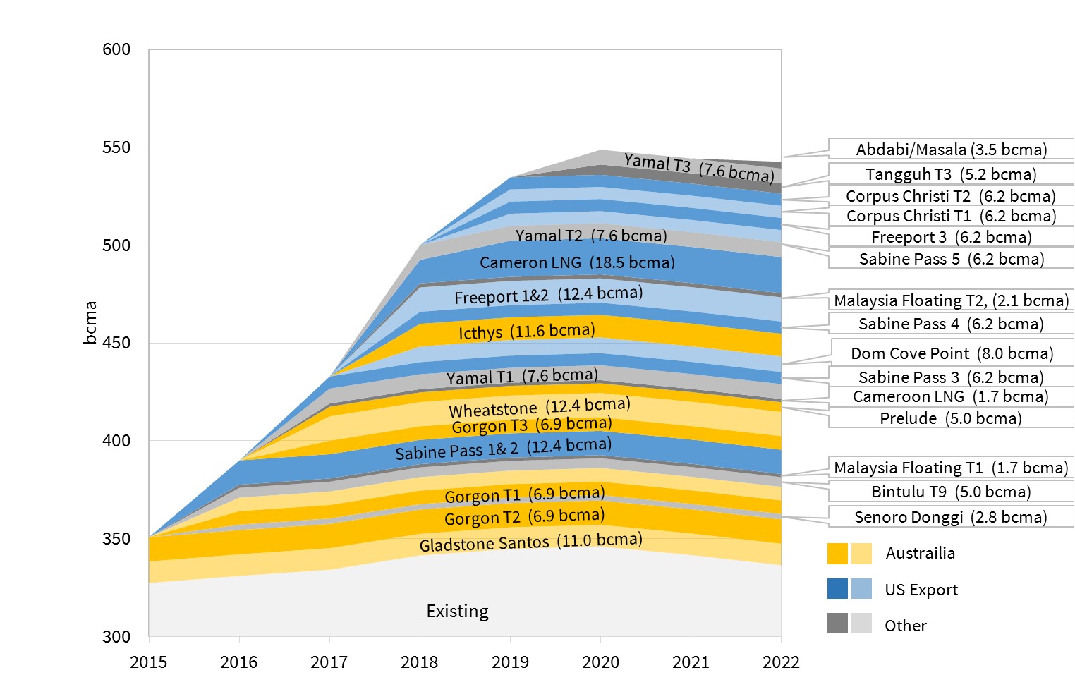
Source: Timera Energy
The impact this supply surge will have on regional markets will be primarily determined by how much LNG Asia is able to absorb.
All eyes on Asian demand growth
The key uncertainties driving future Asian LNG demand growth include the:
- pace and extent of Japan’s nuclear re-start programme
- scale of coal to gas switching in China achieved in line with policy
- affordability of LNG in India (subsidy regime and infrastructure build being key factors)
- aggregate scale of imports in markets such as Pakistan, Bangladesh, Thailand and others where domestic gas production is in decline.
Analysis and judgment can be used to define High and Low future Asian LNG demand scenarios. But it may take a year or two of further evidence before the range of uncertainty can be narrowed. One factor which clouds the picture is the degree of seasonality in Asian LNG demand, in large part driven by the lack of significant gas storage capacity in these markets.
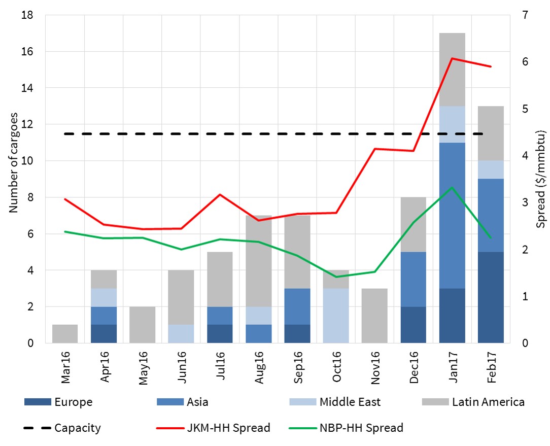
Chart 2 shows monthly Asian LNG import historical data and future trends for both the High and Low scenarios we have defined. Winter 2016/17 saw the impact of an (anticipated) cold Chinese winter and the impact of nuclear capacity offline.
Chart 2 Asian LNG demand (2015 – 2021)
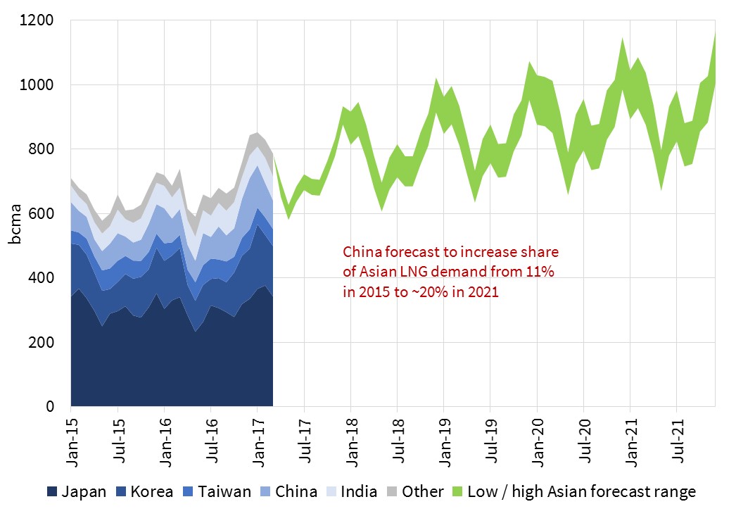
Source: Timera Energy
This resulted in a spike in Asian LNG prices which subsided and re-converged on European hub prices by Spring 2017. Late 2017 Asian import levels should provide a better guide to annual trends (particularly if winter 2017/18 has ‘average’ seasonal temperatures).
Scenario analysis of LNG market balance
Asian demand growth is the most important variable determining the global market gas balance. So we now look at the implications for the wider market of LNG supply growth under the two Asian LNG demand scenarios shown in Chart 2.
Low Demand scenario
Chart 3 shows, for the Low Asian Demand case, global LNG supply compared with non-European LNG demand. In the upper panel, total non-European LNG demand rises to some 520 bcma by 2030. LNG from post FID projects above this demand line is available for Europe. The graph also shows a notional volume of ‘New LNG’ from future (pre-FID) projects from 2025 onwards.
The middle pane shows the European gas market balance, assuming a flat demand level of some 510 bcma. This is met by:
- a) Domestic gas production (including Norway)
- b) pipeline imports comprising North Africa, Azerbaijan and Russia (at take or pay levels)
- c) Russian pipeline gas volumes above take or pay levels (dashed blue)
- d) LNG imports from post-FID projects and
- e) LNG imports from future (pre-FID) projects (assumed to be notionally 180 bcma).
The bulge above the demand line is the ‘LNG glut’ in this scenario. This represents surplus LNG that in not absorbed by ‘business as usual’ demand in Europe. The surplus in this scenario reaches levels of around 60 bcma in 2019 and 2020.
Chart 3 – Low Asia Demand Case LNG Balances
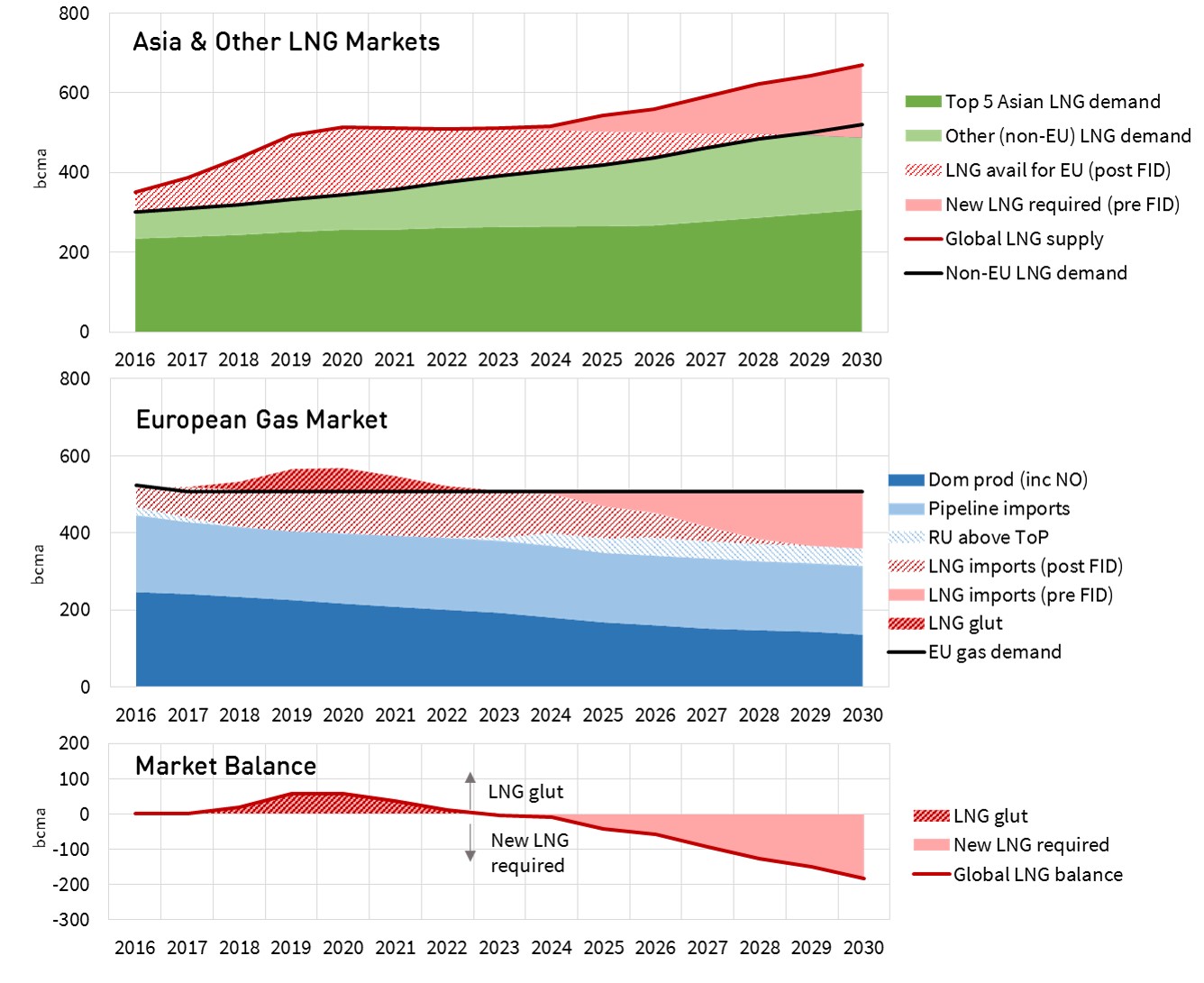
Source: Timera Energy
The lower pane of Chart 3 isolates the glut and the new LNG required from new pre-FID projects. Three points arise from this analysis:
- Although represented as a ‘glut’ – the apparent oversupply of LNG would be cleared by the market through one or more of the following mechanisms: (i) coal to gas switching in the European power sector, (ii) induced additional demand due to lower spot LNG prices in Asia, (iii) potentially a reduction of LNG send-out for coal seam gas – supplied Australian LNG projects and (iv) the curtailment of some US LNG export volumes as the compressed spread between Henry Hub and European hubs (and Asian spot prices) becomes less than the variable costs of the most expensive off-takers.
- As the glut recedes, Europe requires higher volumes of pipeline gas from Russia, who (in this period) are providing the marginal supply tranche into the system and are therefore in a position of ‘pricing power’.
- In anticipation of this re-balancing and consequent higher pricing, new LNG projects gain FID around the turn of the decade and begin producing from 2025 onwards. In Chart 3, the (assumed) mid 2020s wave of new supply is such that it still requires Russian volumes above take or pay levels out to 2030. Consequently Russia retains significant pricing power over European hubs, and through LNG arbitrage, Asian LNG spot prices. It is possible that optimism over future LNG demand trends could lead the industry to ‘overinvest’ in the mid-2020s LNG supply wave, in which case we may see a repeat of the ‘glut’ phenomenon ten years from now.
High Demand scenario
Chart 4 shows the same representations of the global LNG supply and European balance for the High Asian Demand case. In the upper panel, total non-European LNG demand rises to some 635 bcma by 2030. LNG from post FID projects above this demand line is available for Europe. The graph also shows a notional volume of LNG from future (pre-FID) projects from 2024 onwards.
Chart 4 – High Asia Demand Case LNG Balances
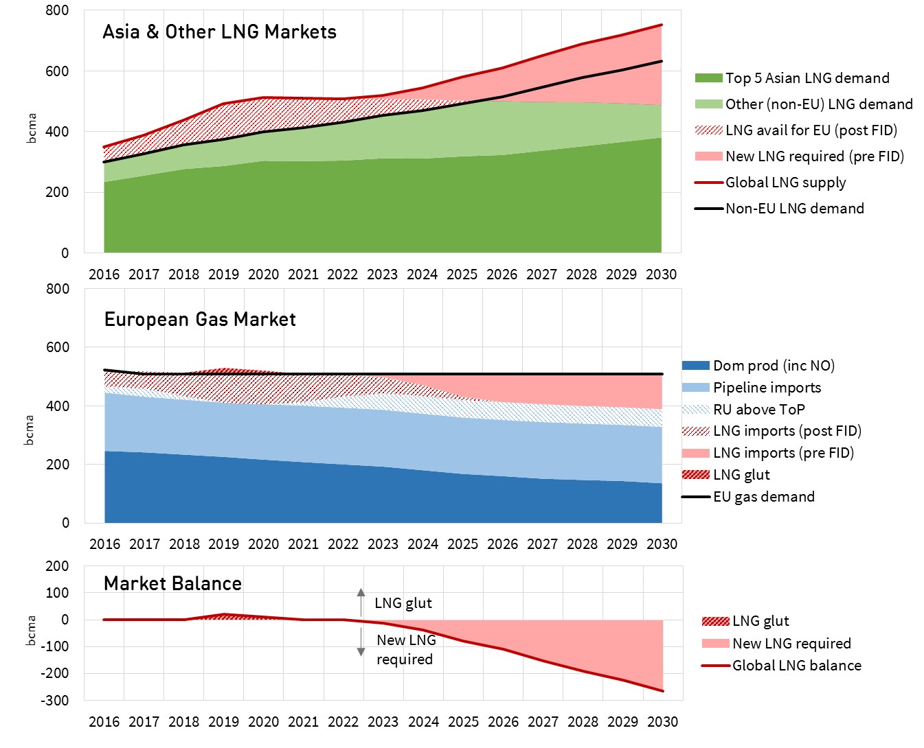
Source: Timera Energy
The middle panel shows the European gas market balance, again assuming a flat demand level of some 510 bcma. As the market in this scenario rebalances earlier and more rapidly, the build-up of Russian volumes above take-or-pay is more emphatic. The ‘LNG glut’ in this scenario is muted: 20 bcma in 2019 and 10 bcma in 2020. The assumed mid 2020’s wave of new LNG supply in this scenario is more significant (270 bcma by 2030), while still leaving Russia with a total of some 210 bcma of pipeline exports to the European regional market.
Implications of scenario analysis
This scenario based analysis of the LNG market balance, forcing attention on the global implication of the LNG cycle, throws up some interesting insights.
Currently industry attention is rightly focused on the period of potential ‘glut’ between 2018 and 2021. But the growth of Asian LNG demand, even in the Low Case, requires near term upstream investment in new LNG project FIDs, by the end of this decade at the latest.
The pace and scale of the next LNG supply wave of the mid 2020s could be comparable to that of the 2010s and even exceed it in the High Case. This again underlines the importance of understanding Asian LNG demand trajectories going forward.
The rise of Russian pricing power in the 2020s is also a feature of both scenarios. This may either be directly or implicitly via an oil-products price linkage. Or it may be via a more strategic targeting of hub pricing through physical volume management.
Time is well invested in better understanding Asian demand growth and Russian price/volume strategy as two critical drivers of LNG market evolution into next decade.
Authors: Howard Rogers, David Stokes & Olly Spinks
Further detail on the themes in article can be found in Howard Rogers’ article: The Forthcoming LNG Supply Wave: A Case of ‘Crying Wolf?’.