Plant closure: drivers of the decision to close

Posted on April 16, 2018January 16, 2020 by David Duncan

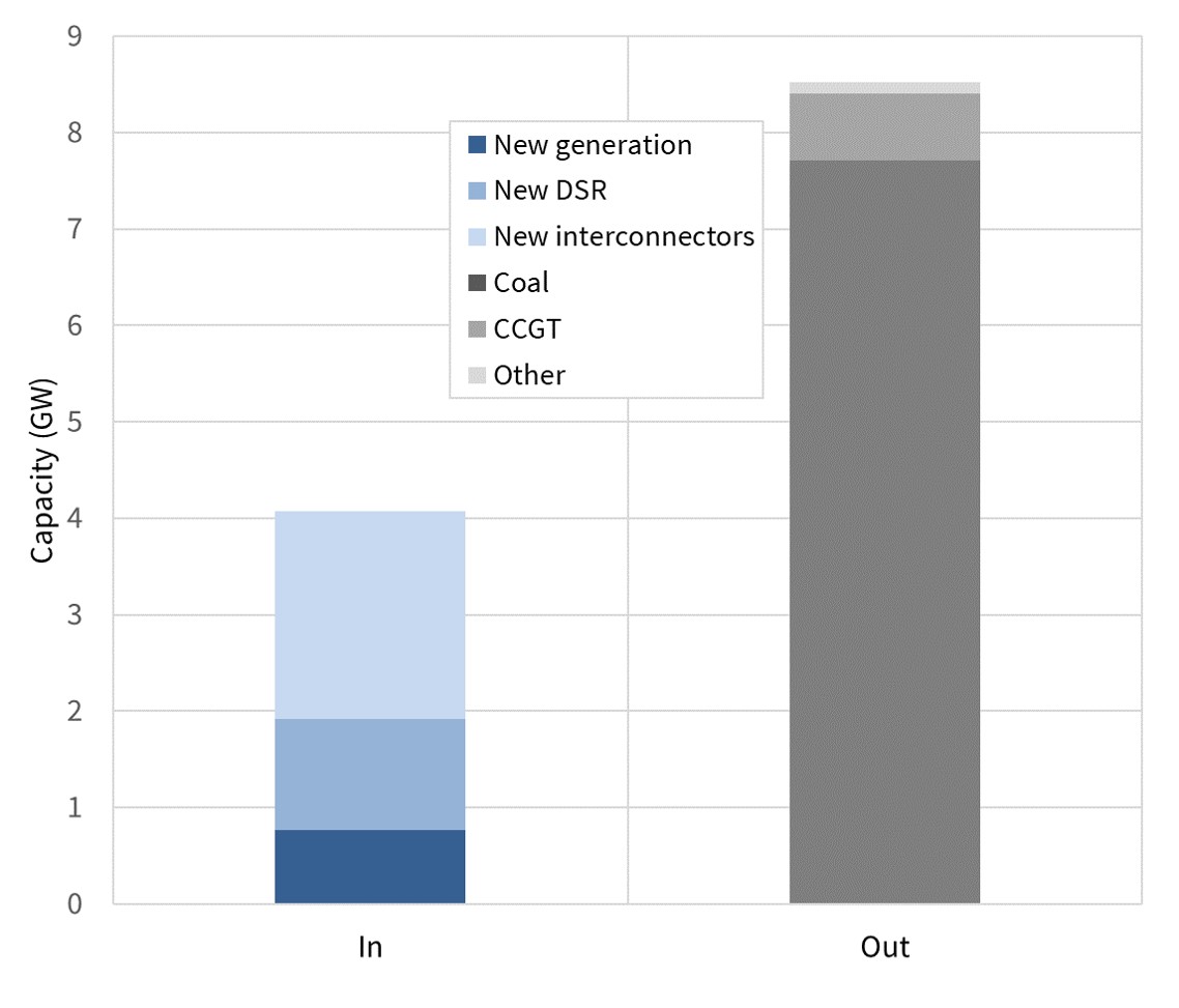
European power markets are facing a demographic issue. Flexible thermal generation capacity is ageing at a faster rate than it is being replaced.

This phenomenon is consistent with the intentions of policy makers as Europe moves towards decarbonization of the power sector. Thermal capacity is steadily being replaced by investment in renewable generation assets.

But new capacity is strongly skewed towards low variable cost and relatively inflexible wind & solar generation. This means the flexibility of remaining thermal power plants is playing an increasingly important role in ensuring power system security of supply.

Low carbon sources of flexibility such as load shifting storage & demand side response are evolving quickly. But evolution of technologies, cost curves and policy support for these low carbon flex sources means that even under optimistic scenarios, Europe will rely on thermal generation flexibility well into the 2030s.

This means that European power markets face a balancing act over the next decade as they progress towards decarbonization. Part of this equation is about investment in new flexible capacity including new low carbon technologies. But capacity demographics are as much about plant deaths as about plant births.

In this context, we focus our next two articles on plant closures. Today we look at economic and other drivers of owners’ decisions to close plants. Then next week we set out a structured investment framework for assessing plant closure decisions.

Closure is more complex than just profitability

Simple investment logic points to plant closure decisions based on profitability. But it is important that profit is viewed from an economic rather than an accounting perspective. By this we mean making decisions based on opportunity costs.

All sunk costs should be excluded from the decision to close a plant. Closure economics should be based on an evaluation of avoidable costs. This is often not straightforward. For example in the context of a UK capacity auction cycle, more costs are avoidable four years ahead of delivery (T-4) compared to one-year ahead (T-1).

All other things being equal, these avoidable costs need to be covered by an adequate level of risk-adjusted revenue, to justify keeping the plant open. Although this concept seems simple, there is usually a complex interaction across a number of value drivers behind it. We summarise these in Table 1.

Table 1: Value drivers of plant closure

Driver	Description	Considerations
Margin uncertainty	Uncertain evolution of wholesale, capacity & balancing/ancillary margins	Large impact on closure economics Probabilistic quantification required Margins need robust risk adjustment Some risks can be hedged Risks increase as load factors decline
Sunk costs	Defining which costs are truly avoidable by closing plant	Important to define over what timescales closure costs become sunk or triggered e.g. rates, insurance, operations & maintenance, redundancy
Cost uncertainty	Elements of cost evolution can carry uncertainty	Many elements of plant cost are stable But some assets face significant uncertainty e.g. potential IED policy costs; transmission charge evolution
Cost reductions	May be options to reduce some plant costs	Assessing options for reducing plant costs can extend asset lives For example, changing station operational patterns & staffing structures; renegotiating O&M contracts
Decomissioning costs	Timing of incurring decommissioning costs can be a significant economic driver	NPV impact of decommissioning cost timing can be substantial, particularly for coal plants
Alternative options	Closure economics need to be consistently assessed against alternatives	Economics of alternatives also need to be quantified, e.g. refurb, mothball, repower Paying an ‘option fee’ to enhance a plant can generate attractive value upside
Other risks	Performance of ageing assets needs to be appropriately risked	Plant performance (outages, efficiency & flex) typically erodes as a plant ages Dispatch profile can significantly increase outage rates (e.g. higher ramping & starts)

Source: Timera Energy

Closure timing and triggers

The precise timing of a closure decision can often be triggered by major cashflow related events that impact the plant. An example of this in a UK, French or Italian market context is exit from a capacity auction (given associated loss of capacity revenue). Other events that can trigger closure include cashflows related to major overhauls, debt repayments and the need to meet changing environmental legislations (e.g. IED capex decisions on coal & lignite plants in Germany).

There can be important practical implications of decommissioning cost liabilities. For example tax and accounting treatment of balance-sheet decommissioning provisions can influence optimization of closure timing. So can the extent to which decommissioning provisions differ from estimated decommissioning costs. Regulatory risk around decommissioning costs is also a consideration, with decommissioning & clean up obligations typically becoming more onerous over time, typically favouring earlier closure.

Closure decisions can also be impacted by codependence with other units on the same site or in the same portfolio. For example, by closing one unit at a four-unit station it is unlikely that a quarter of fixed costs will be saved. Instead, fixed costs are spread over a smaller base and look more expensive from a CFO’s perspective. This may set the bells ringing for the remaining units.

Why decisions can deviate from plant economics

There may be rational explanations for plant closure decisions to deviate from those implied by a purely economic assessment. A good example of this is the portfolio effects of closure. From a strategic bidding perspective in the UK capacity market, portfolio players mays consider the impact of marginal closure decisions of certain plants on the rest of their portfolio. Portfolio value impacts may be driven by the clearing price on the remainder of portfolio generation assets or on costs passed through to integrated retail businesses.

There may also be behavioural or other factors in play that are not obvious from an external economic assessment e.g.

Self-fulfilling prophecy: as closure looms, owners have a tendency to cancel/defer discretionary maintenance, often pushing the plant down an irrecoverable path to closure
Grasping at straws: working in the opposite direction, owners can clutch for excuses to keep a plant (& associated options) alive, even if economics point to closure
Recent acquisition bias: A recent acquirer of a plant may be anchored to pre-acquisition assumptions on market & margin evolution
Last man standing: ‘If everyone else closes first my plant’s value will recover’, or a blind hope variation ‘something will turn up to save us’
Broader perspective Boards can often be reluctant to make politically sensitive or reputationally sensitive decisions around plant closures
Turkey voting for Christmas: a management team working with a portfolio of one plant may not make the same recommendations as a manager with a portfolio of a dozen units

Whether the drivers of closure decisions are economically rational, behaviorally rational or otherwise, these factors all have an important practical impact on plant closure timing. But that does not mean owners should step away from a structured economic assessment of closure decisions.

Large sums of money can be made or lost in optimizing the options associated with a thermal asset approaching the end of its life. We set out an investment decision framework for the assessment of closure vs alternative options in next week’s article, including a practical case study for CCGT assets.

Timera is recruiting power analysts
We are looking for a Senior Power Analyst and a Power Analyst with strong industry experience. Very competitive & flexible packages. Further details at Working with Timera.

Russian & LNG imports: a rebalancing act

Posted on April 9, 2018January 16, 2020 by David Duncan

German and Finnish approval of the Nordstream 2 pipeline over the last two weeks helps pave the way for Russia to continue its role as predominant gas exporter to Europe.

Russian gas will compete with LNG supply to meet growing European import demand in the 2020s. But will Russian or LNG imports replace the seasonal flexibility that Europe is losing from maturing domestic production?

Plenty of Russian gas but seasonal profile is declining

Vast reserves in Western Siberia mean there is no imminent prospect of declining Russian gas production. There is an estimated 100bcma+ of shut in Russian production developed as the result of overly optimistic European gas demand forecasts last decade.

Russian exports to Europe have in fact been steadily increasing since 2015. But as flow volumes have increased, the seasonal profile of Russian imports has declined.

In our last article we set out how maturing production was causing a decline in seasonal flex from the UK, Netherlands and Norway. In the case of Russia, loss of seasonal flex is driven by changing flow routes and strategy rather than upstream issues.

Gazprom has made a clear strategic decision to bypass the traditional Ukrainian flow route to the extent that capacity is available on other routes. This strategy is set to continue given:

Significant historical transit losses and ongoing political tensions with Ukraine
Nordstream 2 facilitating additional flow volumes via northern routes into Europe.

As part of this strategy, Russia has also substantially reduced its usage of Ukraine’s vast gas storage assets. This has effectively eroded the provision of flex from Ukrainian storage to the European gas market. The loss of seasonal profile from Russian flows has been reinforced by Gazprom more actively marketing uncontracted volumes at European hubs across the summer months (having overcome its previous aversion to selling at spot prices).

The reduction in the seasonal flow profile of Russian imports can be seen in Chart 1.

Chart 1: Russian flow volumes by key routes to Europe this decade

LNG imports providing the wrong sort of seasonality

As domestic production declines, incremental LNG imports will be the other key source of supply growth into Europe. LNG flows reflect regional supply & demand balances and price spreads. This means LNG provides a very different sort of flex to Russian gas.

The LNG market can deliver Europe large incremental volumes of gas at the right price. But the supply chain for LNG is more complex than for pipeline supply. And it takes longer to respond to market price signals, typically from 2-6 weeks to deliver a material increase in volume.

There are however growing structural trends in the way LNG flows into Europe. An increasing shortage of domestic storage in Asia (particularly in China) is causing flexible LNG cargoes to be diverted away from Europe across the winter. This dynamic has been clear over the last two winters as Chinese LNG demand has surged.

A similar logic tends to cause surplus LNG to flow into European hubs across the summer months. In other words, European LNG imports are increasingly displaying a counter-seasonal profile which is compounding the loss of seasonal shape from domestic production.

Flex market rebalancing

In our last article we set out why Europe faces an unambiguous decline in seasonality from domestic production. The earthquake induced pace of reductions in Groningen production, now targeted to cease production by 2030, is accelerating this dynamic.

In today’s article we have explained why structural trends driving Russian and LNG import profiles are also reducing the seasonal shape of flows into Europe.

For the last decade the European gas market has experienced an oversupply of seasonal gas flexibility. This was the result of weaker than expected gas demand, overbuild of storage and improved optimisation of existing portfolio flexibility.

However investment in seasonal flexibility has dried up at the same time structural trends are eroding existing seasonal flex. Over the last five years, seasonal price spreads at European hubs have been crushed towards the variable cost of cycling seasonal storage assets (1.0-1.5 €/MWh). It may be complacent to assume that spreads remain at this level for the next five years.

European production flex is declining fast

Posted on March 26, 2018January 16, 2020 by David Duncan

Europe faces a structural decline in domestic gas production. Domestic output (excluding Russia) is set to decline from 252 bcma in 2017 to 150 bcma by 2030.

This trend of declining production is well understood. But the associated decline in supply flexibility and seasonality of production flows is less so. Rapid declines in Groningen output and maturing Norwegian production are combining to erode domestic supply flexibility in Europe.

In this week’s article we consider the scale of lost domestic production flexibility. Then in our next article we look at how changes in Russian export strategy and flow routes are also impacting supply flexibility.

Breakdown of key domestic supply sources

Three main sources of domestic production have historically provided substantial seasonal flexibility to the European gas market. But maturing production, ageing assets and falling upstream capex investment are reducing both the level and seasonality of flows.

Netherlands

Earthquake related production cuts have reduced Dutch gas production by 70% since 2013. This year’s latest 12bcma cap has also substantially eroded Groningen’s seasonal production profile.

Prior to 2013, the Netherlands historically provided a seasonal swing of 6-7 bcm of monthly output from highest winter month to lowest summer month as illustrated in the top panel of Chart 1. That will fall to less than 1 bcm swing under the new cap.

Chart 1: Historical & projected monthly Dutch gas production (2010-30)

Norway

Norwegian production has plateaued and is set to steadily decline next decade. Norway provides 3-4 bcm peak winter to trough summer month swing. This is likely to fall to under 2bcm later next decade as can be seen in Chart 2.

Chart 2: Historical & projected monthly Norwegian gas production (2010-30)

Norwegian seasonal flexibility has played a key role in ‘backfilling’ the loss of Rough storage in the UK. That has reduced seasonal profile of flows to the Continent.

As well as seasonal flex, Norway provides important daily deliverability flexibility, particularly into the UK gas market. Recent declines in Norwegian upstream capex spend rates are set to impact provison of flexibility over the next 5 years. Reduced performance from the large Troll field could significantly curtail Norway’s supply flexibility in the 2020s.

UK (& other)

The UK has historically been Europe’s third key domestic producer. However UK production declines over the last 15 years have already substantially reduced supply flexibility. The UK peak to trough monthly swing is less than 1 bcm and will decline further with production next decade.

This pattern is also true across other European domestic production (e.g. in Germany, Italy, Poland & Romania) which has a relatively flat profile.

The upshot of declining domestic supply flex is that Europe is rapidly becoming more dependent on imported flexibility. That leads us to look at Russian supply flexibility in or next article. But we will be taking a one week break over Easter first.

NW Europe’s flexible capacity crunch

Posted on March 19, 2018January 16, 2020 by David Duncan

The luxury of oversupply

There has been a structural oversupply of capacity in North West European power markets this decade (with the notable exception of the UK). Excess capacity has been the result of slower than expected demand growth. This has been exacerbated by an overbuild of thermal assets, particularly new coal and CCGT plants in Germany and the Netherlands.

Strong policy support for renewable generation has seen wind, solar and biomass capacity delivered into power markets which already have excess thermal capacity and adequate flexibility to absorb intermittency. Structurally oversupplied markets have shaped policy decisions and investor attitudes to deploying capital.

Retirements pipeline changes the landscape

The NW European power market balance is set to substantially change across the next 5-7 year due to:

Regulatory driven nuclear closures, for example:
1. 10GW in DE by 2022
2. 6GW in BE by 2025
IED & national policy driven closures of coal units, for example:
1. 12GW in UK by 2025
2. ~10GW in DE by 2025 (IED dependent)
3. 3GW in FR by 2022
4. 5GW in NL by 2030
Ageing gas plants will need major lifetime renewal capex or close by 2025, for example:
1. ~10 GW in Germany
2. ~9 GW in UK

Cumulative projected thermal capacity retirements by country are shown in Chart 1, based on currently announced policy measures.

Chart 1: Projected NW European thermal capacity retirements

Source: Timera Energy

These closures will significantly tighten the NW European capacity balance as well as removing substantial volumes of dispatchable flexible capacity.

Policy makers are not blind to this challenge. In February the EU approved a further 6 capacity payment mechanisms (DE, BE, IT, FR, PL & GR). But despite new policy measures there is not yet a compelling investment case to support delivery of new flexible capacity (UK aside).

The requirement for new capacity is clear from a security of supply perspective. But the price signals that will support capacity investment are less clear.

A capacity mechanism tour of NW Europe

UK:

Necessity is the mother of intervention. The UK power market tightened over the first half of this decade as thermal capacity retired. As a result the UK implemented a capacity market that has delivered significant volumes of new flexible capacity.

Capacity investment has been underpinned by 4 year ahead auctions of up to 15 year capacity agreements for new builds i.e. a clear capacity price signal that supports commitment of capital. This approach has not been replicated in other NW European markets.

France:

French security of supply is underpinned by its 63GW nuclear fleet. Despite political rhetoric, there is unlikely to be substantial net closures of French nuclear capacity before 2030. Nuclear is complimented by significant hydro flex and high levels of interconnection. Flexible capacity retirement volumes are likely to be relatively low over the next decade and will predominantly be replaced by a ramp up in renewable capacity.

The French implemented a supplier obligation based capacity market in 2017, with annual capacity payments. In practice this mechanism is likely to be more focused on retaining existing capacity than supporting structural investment in new flexibility. However the French government have provided specific support for new thermal capacity (a CCGT project to alleviate constraints in Brittany) and the newly approved French demand response mechanism may flush out some DSR flex.

Belgium:

Belgium is a step closer to the UK in terms of market tightness. But it is a relatively small market which is very well interconnected (6GW of links with FR & NL). Belgium’s major issue is replacement of 6GW of ageing nuclear capacity between 2022-25. The government and TSO are aiming to do this without a step change in dependency on imported power.

The EU state aid commission approved a Belgian strategic reserve mechanism in Feb 2018. This is focused on an emergency reserve to retain ageing thermal units (that would otherwise close). It may also help some smaller distributed capacity, but it is unlikely to structurally solve the nuclear replacement issue. That suggests that wholesale prices and volatility are set to rise.

Netherlands:

Thermal capacity overbuild has been most acute in the Netherlands. The first half of this decade saw an almost masochistic competitive battle between utilities and independent developers to deliver new capacity volume at the expense of margins. This wounded thermal plant owners, but excess capacity has dampened security of supply concerns for the Dutch government.

The Netherlands has a relatively young and flexible thermal fleet dominated by CCGTs. Ongoing proactive support for renewables is set to fill most of the capacity gap from retiring plants. This means that intermittency will play a more important role in the Dutch supply stack going forward. But capacity developers will need to look to the wholesale market for investment price signals.

Germany faces the biggest capacity challenge

Germany anchors the network of NW European power markets. German thermal capacity dominates regional price setting. Swings in renewable output are also increasingly drawing on regional flexibility, as Germany moves towards its target of a 65% renewable energy share by 2030. The challenge Germany faces is being exacerbated by substantial closures of thermal capacity.

After the Fukushima disaster, Germany decided to close its remaining 12GW of nuclear capacity. We are sceptical of the closure logic from an emissions perspective. But the German government is effectively implementing the plan, with 9.4GW of remaining capacity to close by 2022.

Germany is also likely to close an estimated 10GW of coal and lignite units by 2025. This includes 2.7GW of lignite units currently ring-fenced in a climate reserve. It also covers a number of older coal units that breach IED NOx limits. IED driven closures of coal & lignite may rise to 20GW by 2030, although volume uncertainty remains given potential capex spend to mitigate emissions on some units.

Germany also has an ageing gas plant fleet. CCGTs typically require major lifetime renewal capex to avoid closure at around the 25 year mark (although exact timing is dependent on run hours, technology configuration and operational patterns). Another 10GW of gas-fired units will reach this point by mid next decade, likely resulting in substantial gas plant closures.

Given the scale of thermal closures, Germany faces a structurally different problem to other markets such as France and the Netherlands. German capacity maths does not add up without substantial investment in new flexible capacity. The strategic reserve mechanism that has just been approved by the EU does not appear to solve this problem.

Implementation of the strategic reserve is planned for 2019. The reserve allows payments to existing thermal units that would otherwise close, but support is capped at 2GW of capacity. This compares to 10.4GW of capacity contracted for Winter 17-18 under the current network reserve mechanism (although the reserve requirement will fall next winter once the German-Austria market split is implemented).

The reserve measures Germany has pursued to date are focused on retaining existing capacity, not delivering investment in new flexibility i.e. slowing exit rather than increasing new entry. That points to Germany also heading down the path of sharper wholesale market and balancing services price signals. This may support a recovery in the value of existing flexible power assets. It also pushes market price risk onto investors in new flexible capacity, who will need to see a path to higher expected returns in order to deploy capital.

Will LNG bunkering transform the LNG market?

Posted on March 12, 2018January 16, 2020 by David Duncan

Tightening emissions standards are supporting structural growth in the uptake of LNG as a shipping fuel. Europe has led this transition, dominating the fleet of existing vessels and associated infrastructure. But growth is now accelerating globally.

LNG bunkering has created considerable excitement as a new source of demand in the LNG market. Today we look at the drivers and potential scale of LNG demand growth from shipping.

Emissions regulations driving change

In 2016 the International Maritime Organisation (IMO) announced requirements for significant reductions of marine fuel sulphur by 2020. Under the new provisions, marine fuel used in ships will have to have a sulphur content of no more than 0.5% versus the current limit of 3.5%. Emissions standards have already been tightened to a cap of 0.1% for designated Emission Control Areas (ECA’s) for coastlines in the US and Northern Europe.

The IMO 2020 regulations will require ship owners to decide whether to:

continue using high sulphur fuel oil and add scrubbers/exhaust gas cleaning systems or
switch to low sulphur fuel options i.e. distillates or LNG.

Tighter emissions standards are acting as a tailwind for LNG-fuelled vessels.

Growing fleet & order books

There is an existing global LNG-fuelled fleet of around 120 vessels. More than 60% of these are European based. LNG consumption of the current fleet is around 0.25 mtpa.

The fleet has been growing recently at a rate of about 20% a year, with a current global order book of a similar size to the existing fleet.

While this headline growth rate is impressive, understanding different vessel classification segments is important for estimating implications for LNG demand growth. This is the primary reason for uncertainty in forecasts of future bunker fuel LNG consumption.

Passenger ships account for around 35% of existing and ordered vessels. Demand here is driven by leading cruise ship operators placing orders to help avoid emissions constraints in city ports.

But the strongest recent growth in vessel demand has been for larger LNG-fuelled tankers and bulk carriers. In addition to an in-service fleet of 19 vessels, 10 chemical/product tankers have been ordered. Four Aframax ice class oil tankers have been ordered by Socomflot which will be taken on charter by Shell.

The LNG-fuelled marine industry focus is shifting from Norway and the Baltic region northern Europe and North American trade. Four of the LNG fuelled vessels in operation already operate globally and 22 newbuilds are also destined for global trade.

Oil and gas offshore industry service vessels rank second in terms of LNG uptake. However, this is unlikely to be a major source of significant future growth.

Higher growth is expected in the tanker, car/passenger, cruise and container segments. Container ships are well suited for LNG fuel, with fixed routes and a high fuel consumption to earn back the additional investment.

In late 2017 Total agreed to supply French shipping firm CMA CGM with around 300,000 t/year of LNG bunker fuel for 10 years from 2020 – the largest such contract to date. CMA CGM has ordered nine 22,000 twenty-foot equivalent unit (TEU) container ships with LNG fuelled engines. The French government is planning to support development of LNG bunkering infrastructure at the country’s ports.

LNG bunkering infrastructure

LNG bunkering infrastructure is currently concentrated in areas affected by the existing tighter ECA emissions standards and with access to LNG from regas or liquefaction related storage tanks and port facilities. These include:

North west Europe (for example, in the ports of Rotterdam, Stockholm and Zeebrugge)
The US Gulf and East coast (including the ports of Jacksonville and Fourchon)

These make up the bunkering nodes around which a global LNG-fuelled shipping industry will be developed.

Key Asian ports serving deep-sea shipping routes are in the process of establishing LNG bunkering facilities and looking to co-ordinate activities with their European and North American counterparts. This is most evident in the infrastructure being developed by Singapore and in ports in eastern China, for example Ningbo-Zhoushan, the world’s biggest cargo port.

Chart 1: Global infrastructure for LNG bunkering

Source: DNV.GL

Current EU policy requires at least one LNG bunkering port in each member state. About 10% of European coastal and inland ports will be included, a total of 139 ports. Coastal port LNG infrastructure will be completed by 2020 and for inland ports by 2025.

There are several ports under development in North America, mostly in the south east, the Gulf of Mexico and around the Great Lakes, but also for ferry and deep-sea operations in the Pacific Northwest.

China is extending LNG bunkering infrastructure from inland waterways to coastal areas and is expected to be able to service the LNG demand of all vessel types. South Korea offers LNG bunkering in the port of Incheon and is considering a second facility in Busan. Elsewhere in Asia, in addition to Singapore, Japan and Australia are also working to develop LNG bunkering facilities.

Potential impact on global LNG demand

The IEA, in their 2017 World Energy Outlook, see the use of LNG replacing heavy-fuel oil as a bunker fuel providing around a 25% reduction in CO2 emissions. Notwithstanding the challenges in forecasting LNG bunker fuel outlined above, the IEA make the following projections for their ‘New Policies Scenario’ and a ‘Sustainable Development Scenario’. In the latter it is assumed that the IMO limits on sulphur are further tightened – hence the increased LNG consumption in bunkering.

Chart 2: IEA LNG marine fuel demand forecast (bcma)

Source: IEA World Outlook 2017

To put these LNG bunkering demand numbers in context, they are equivalent to the projected demand growth of one of the larger emerging Asian buyers e.g. Thailand or Pakistan.

As such LNG bunkering is an interesting demand growth trend to keep an eye on. But it is unlikely to have a transformational impact on global LNG market demand.

Gas market explodes into action

Posted on March 5, 2018January 16, 2020 by David Duncan

Cold weather across North West Europe sparked a surge in gas price volatility last week. The epicentre of system stress was the UK gas market. But the parallel spike in NBP and TTF prices reflected a UK and Dutch fight for gas across the interconnectors, with price shocks reverberating across the European gas hub network.

In today’s article we summarise the events that culminated in one of the sharpest bursts of gas price volatility this decade. We also touch on how this impacted other European hubs and the UK power market. But more importantly we consider the potential implications for policy, supply flex value and the re-pricing of portfolio risk.

Anatomy of a gas market shock

System stress built over the course of last week as temperatures plummeted across NW Europe. The impact of the arctic blast peaked on Thursday where the UK TSO (National Grid) forecast a 50 mcm shortage of gas for the day and issued its first ever gas deficit warning.

Demand reached its highest level since 2010 on Thursday (410 mcm). There were also significant weather related supply infrastructure outages (Kollsnes 16 mcm, SEGAL 18 mcm & a temporary halt on South Hook terminal send out). This saw the UK’s first real test of system deliverability in a post Rough environment.

Within-day prices were elevated across the day, peaking at an unprecedented 450 p/th on Thursday evening. Grid was actively buying back gas from large industrials at elevated prices to help balance the system.

Within-Day prices at the Dutch TTF hub also rose above 120 €/MWh as Europe’s two primary hubs battled for limited gas supply. Other hubs across Europe were caught in the price uplift, although most traded at a significant negative basis to NBP and TTF as we showed in our Snapshot column on Fri. The exception was PEG Nord with Northern France facing a shortage of gas driven by declining LNG send out and falling Norwegian deliveries.

Chart 1 illustrates how UK supply flex responded to the sharp jump in price signals. Storage withdrawals (~80 mcm) and LNG tank send out (~60-80 mcm) played a key role in plugging the gap. The ability for LNG terminal send out at this rate is typically restricted to a couple of days given limited inventories. Interestingly the IUK interconnector was importing at lower than normal rates as TTF price rises kept pace with NBP.

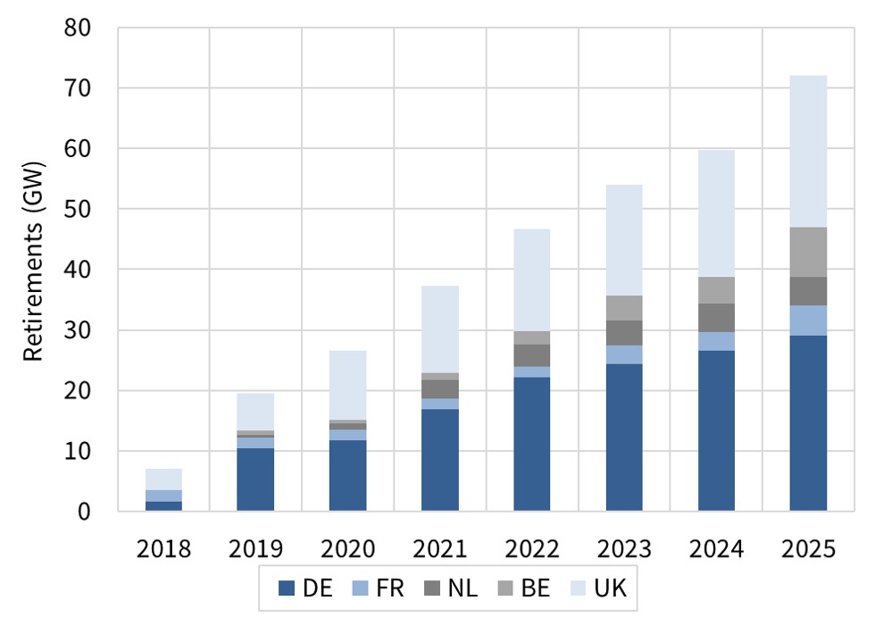
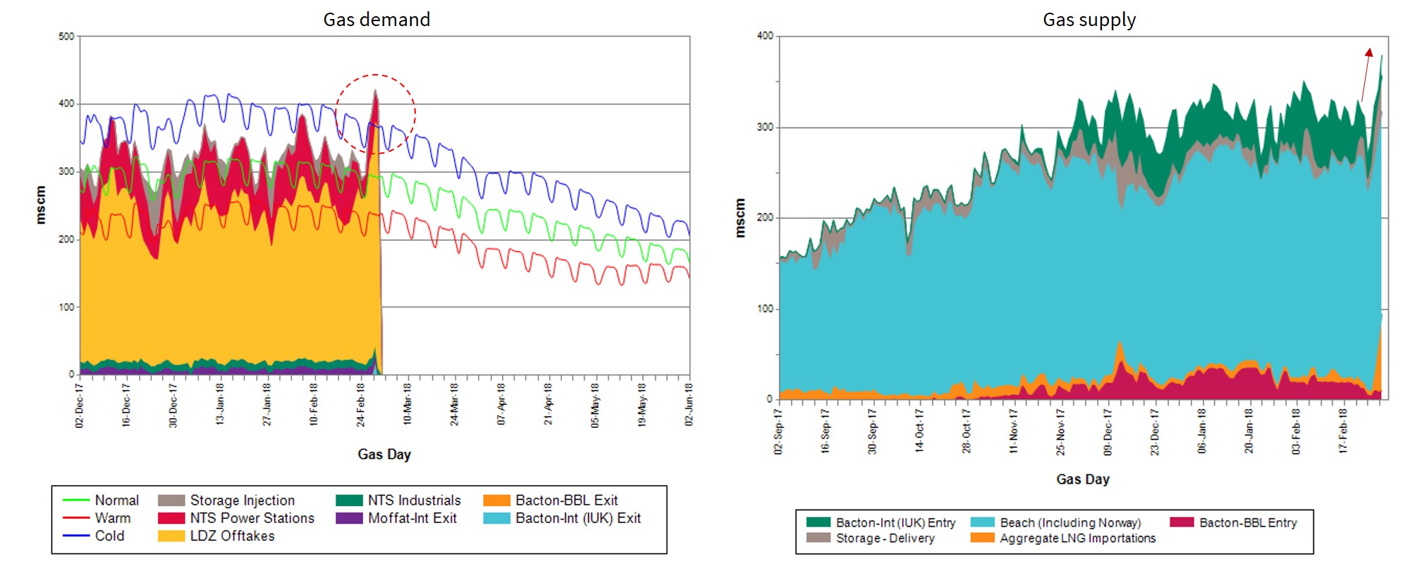
Chart 1 Evolution of UK gas supply across key sources Source: National Grid

These short term fireworks had little impact on NBP and TTF forward curves beyond the horizon of the current cold spell. The fact that the impact of system stress was focused on prompt prices is a sign of a well functioning commodity market.

UK power market reaction

UK power prices leapt in sympathy with gas prices, but market stress was actually less acute. A liquid gas market ensures direct pass through of higher spot gas prices into power prices. Very high gas prices saw power prices jump above 100 £/MWh later last week, even in the context of a market that had capacity headroom to spare.

Stress in the power market was highest on Thursday morning when unusually cold weather impacted the ability of several large CCGTs and a nuclear plant to start. But elevated gas prices ensured that CCGTs were at a significant variable cost disadvantage to coal units. This saw 11GW of coal capacity running baseload which along with healthy wind output helped to cap system tightness.

The events of last week are a reminder of several evolving power market dynamics:

Gas volatility: As the UK gas market becomes more import dependent, rising gas price volatility is set to translate into higher power price volatility, given the price setting dominance of gas-fired power plants.
Coal closures: The replacement of 11GW of coal capacity with other flex is causing a major transition in price setting dynamics to the right of the supply stack (e.g. GTs and engines have much higher variable costs than coal).
Outages: Flexible infrastructure outages tend to be correlated with market shocks (e.g. due to cold weather), particularly for ageing assets.

Policy implications of this market shock

The key takeaway from the events of last week is that markets worked as they should. Security of supply was maintained through a period of major system stress driven by a combination of very high demand and supply outages.

In the short term, gas supply is inelastic (unresponsive to price). This means temporary market shocks cause extreme short term price movements to ensure the balance of supply and demand. This price volatility is evidence of well functioning markets rather than system failure.

The UK gas market in particular needs investment in new deliverability flexibility after the closure of Rough storage (as we have written about previously). Spot volatility is the price signal required for investors to commit capital.

Expect a repricing of portfolio risk & supply flex

While recent gas market tightness does not constitute market failure, it is likely to trigger a re-pricing of ‘tail risk’. A low volatility environment has steadily eroded risk premiums over the last five years. But market shocks are set to increase in frequency and magnitude as import dependency increases. The extreme nature of recent price moves reinforces the portfolio insurance role of supply flexibility.

Energy supply is a high volume, low margin business that is vulnerable to irregular market shocks. A number of new entrant suppliers have already fallen victim to market price risk this winter. More may follow after last week. As the new entrant supplier model matures, demand for flexible insurance products (e.g. price caps) is set to rise significantly.

This dynamic is already being anticipated by larger gas portfolio players. A re-pricing of risk is reflected in a step change in demand for gas supply flexibility since the closure of Rough. Interest here is twofold: (i) to cover own portfolio risk and (ii) to enable the origination and sale of insurance products to new entrants and less sophisticated players.

The value of flexible gas supply infrastructure is in a cyclical trough. But increasing portfolio demand for gas supply flex points to recovering prices ahead for storage and regas assets.

Deconstructing LNG shipping costs

Posted on February 26, 2018January 16, 2020 by David Duncan

Shipping costs seems like a relatively obscure topic. Yet one of the most popular articles in our blog archive is a 2013 article that provides a breakdown of LNG shipping cost components.

So why are people interested? The delivery of LNG cargoes is increasingly being optimised against spot price signals. Margin opportunities in moving LNG between regions depends on the cost of transportation. This means that shipping cost differentials have become key drivers of LNG flows & regional price spreads.

Given that context we are publishing an updated version of the article to address a number of developments over the last 5 years.

Cost component breakdown

The following factors are the key determinants of shipping costs from point A to B.

Chartering fee: This is the payment for securing access to shipping capacity by chartering a vessel. There are broadly three ways to access shipping capacity: (1) own vessel capacity (2) time charter and (3) single voyage or spot charter. Spot charter rates are generally higher and certainly more volatile than longer term time charter rates. Strong Asian demand across this winter has seen spot charter rates rise to between $70-80k per day for 160,000 mcm vessels.

Brokerage: Vessel charters are typically arranged through specialist brokers and attract a 1-2% fee.

Vessel type: Historically most LNG vessels were powered by Steam Turbines (ST) which can burn a combination of heavy fuel oil (HFO) and boil-off gas in their boilers. Modern diesel engines have replaced STs in new vessels delivered over recent years. Dual / Tri Fuel Diesel Engine (D/TFDE) can also burn a mixture of HFO and boil-off gas but are much more efficient (reducing fuel costs). Vessel size is also an important determinant of voyage economics and cost. The most common size is around 147k to 160k m3 but larger vessels are also available between 210k m3 (Q-Flex) and up to 260k m3 (Q-Max).

Fuel cost: The voyage fuel or ‘bunker’ consumption is directly proportional to the distance and speed of the vessel. This is typically the second largest cost component after the chartering cost. The different propulsion mechanisms and fuel burn options add some complexity. Most LNG vessels can burn fuel oil, boil-off gas or a blend of both in their boilers. As a result the calculation of fuel cost is closely tied to that of boil-off gas.

Natural boil-off occurs at a rate of ~0.1-0.2% of inventory per day and at times boil off is forced above this level to further reduce fuel oil requirements. Some modern LNG vessels also have the ability to re-liquefy boil-off gas, keeping the cargo whole (while running on more fuel efficient diesel engines).

LNG vessels also require a minimum inventory (called “heel”) to keep the tanks cool (and fuel for unladen voyages if running on boil-off). Calculation of direct fuel consumption is fairly straightforward but the opportunity cost of LNG boil-off is also an important consideration.

The choice of fuel blend influences achievable speeds e.g. around 14 knots running on boil-off alone compared to around 19 knots running on HFO or forced boil-off. Speeds in turn can also have implications for charter costs and ability to reach a destination in time to capture premium spot prices.

Port costs: The components and level of the costs of loading and unloading at ports can vary widely depending on location. For example, ports in less stable regions can levy large security charges associated with ensuring the safety of the vessel.

Canal costs: Transit costs have to be paid for using the cross-continental Suez and Panama canals. Canal transit costs are in the region of USD 300-500k per transit. The Panama canal widening project, completed in 2016, has opened up the route to the majority (~80%) of LNG vessels. Previously only a small fraction of the LNG tanker fleet could squeeze through. This is an important development for US export projects as the canal transit reduces the distance and cost from the US Gulf Coast to premium Asian markets.

Insurance costs: Insurance is required for the vessel, cargo and to cover demurrage (liabilities for cargo loading and discharge overruns).

Putting the pieces together

Once you have reflected the components above in a shipping cost calculator, it is a relatively simple analytical exercise to estimate shipping costs. In Chart 1 we show OIES analysis by Howard Rogers (a senior member of the Timera gas team) illustrating the cost breakdowns of different vessel types.

Chart 1 DFDE vs ST shipping cost estimates on major routes

Source: Howard Rogers; assumptions: Charter rates: DFDE $60k pd, ST $47k pd. Speed DFDE (on HFO) 19 knts vs ST (on boil-off) 14 kts. HFO price: 380 $/tonne.

Optimising shipping logistics is a challenging problem e.g. choice of vessel type, propulsion & speed. But across a range of complex options, route costs are broadly the same as illustrated by DFDE vs ST costs in Chart 1. This is not a total coincidence as charter rates tend to broadly adjust to equalise shipping costs given a significant degree of vessel substitutability.

Market interest in shipping costs extends beyond optimisation of cargo logistics. A high proportion of new supply being commissioned over the 2016-21 period consists of flexible FOB cargoes (dominated by US exports). At the same time traded LNG market liquidity is increasing.

These forces mean that regional price differentials and LNG portfolio value opportunities are increasingly being driven by shipping costs. That is bringing the behaviour of cost components into sharper focus.

Implications of UK capacity auction results

Posted on February 19, 2018January 16, 2020 by David Duncan

There have been genuine reductions in the costs of flexible capacity over the last 12 months. These have been supported by falling costs of capital as investors target UK power infrastructure. But capacity cost reductions had little to do with an auction clearing price of 8.40 £/kW.

The auction result was instead driven by lower than expected exit price levels for older coal & CCGT plants. These are hard to reconcile with the gap between current unit margins and fixed costs. But low bids suggest an unwillingness from owners to close older plants, whether for ‘strategic’ or other reasons.

A range of analysis has been published on why the T-4 auction cleared at 8 £/kW. In today’s article we focus instead on implications of the auction result. We consider what it means for evolution of the capacity mix, market pricing dynamics and asset investment.

Capacity mix changes

Successful and unsuccessful capacity in the auction are summarised in Chart 1.

Chart 1: New and exited capacity from 2021-22 T-4 auction

Source: Timera Energy, National Grid

What’s in?

2.2GW of interconnector capacity was successful across three projects, Eleclink (UK-FR), NEMO (UK-BE) and IFA2 (UK-FR). 0.8GW of new generation capacity was dominated by distribution connected gas engines. 1.2GW of new DSR was also strongly influenced by engines and batteries behind the meter.

What’s out?

8.5GW older existing thermal capacity exited the auction. 7.7GW of coal units, 0.7GW of older CCGTs and 0.1GW of coal plant GTs and engines.

These exits will have some important near term implications for coal plant closures:

Eggborough (1.8GW) has announced closure this year after exiting the T-1 auction
Fiddlers Ferry (1.7GW) and Cottam (1.8GW) will likely close after the 2018-19 capacity year given these plants have no capacity support beyond.
Aberthaw (1.5GW) will likely close after 2020-21 given no agreement beyond.
West Burton (1.8GW) has no capacity agreement in 2019-20 but does have one in 2020-21. This plant is likely to remain open until early next decade hunting T-1 support, but in doing so may supress T-1 prices.

Beyond 2021-22 the UK coal fleet is likely to be reduced to the IED compliant Drax coal units (1.2GW) and Ratcliffe (1.8GW). Based on current market conditions the UK may well achieve its targeted closure of all coal stations prior to 2025, on an economic basis alone.

Market pricing impact

The capacity mix changes from this year’s auction set up a major shift in the UK supply stack:

Removal of large grid connected coal assets from the middle of the stack
Replacement of this capacity with:
- high variable cost engines/DSR (at the far right of stack)
- interconnectors whose pricing/volume depends on conditions in foreign markets

The replacement of mid-merit with peaking plants, accelerates a trend established in the previous three auctions. While it fulfils the government’s goals in a capacity accounting sense, it will have some important implications for wholesale market pricing dynamics.

Changing stack shape is set to support super peak prices. The removal of coal units means prices will more often need to rise to bring on gas engines during periods of high net system demand. This is likely to increase the peak/offpeak price ratio as well as supporting spot price volatility.

The competitive position of new interconnectors in the supply stack depends on price levels in foreign markets. Under normal market conditions, the interconnectors will tend to import cheaper power from the Continent. But Winter 2016/17 has shown that flows can dry up or reverse during periods of UK system stress, if these coincide with stress in Continental power markets (e.g. FR, NL, BE).

3GW (nameplate) of new interconnector capacity will support price convergence with the Continent. This will make it much more difficult for other new interconnector projects to follow.

The capacity mix transition from grid to distribution connected assets also poses challenges in balancing services markets. For example reductions in:

active provision of flex in the Balancing Mechanism
provision of ancillary services

None of these are insurmountable, but they bring National Grid’s current review of balancing services procurement into focus.

Asset investment implications

Investors are keenly aware of a key policy question arising from the auction result. Are the regulatory authorities and National Grid (as TSO) comfortable with the type of capacity being delivered by the market?

If the answer to that question is no, then watch out for potential policy changes that (i) support new CCGTs and/or (ii) reduce the competitiveness of engines/DSR. For example:

A rule change to limit cashout price chasing would present a major challenge to gas engines
Toughening of DSR performance standards would erode competitiveness of behind the meter flex.

Four capacity auctions have now passed and a large new CCGT project is yet to succeed. However behind the scenes new CCGT costs continue to fall, due to a combination of rising efficiency, falling turbine costs and reductions in cost of capital. Despite this it will be difficult to build new CCGTs with capacity prices below 20 £/kW. This means new CCGT projects remain queued to cap any capacity price rises above 25 £/kW.

More efficient and flexible existing CCGTs are set to benefit in the wholesale market from the supply stack transition. The increasing influence of higher variable cost peaker/DSR capacity supports CCGT margin rents. But an 8 £/kW capacity price is a tough price to absorb for these benefits.

A single digit clearing price has caught owners of existing CCGTs by surprise. It brings brings future bidding strategy & closure decisions sharply into focus for older, less efficient and less flexible CCGTs.

These older CCGTs have fixed costs of 20-25 £/kW. On a risk adjusted margin basis it makes no sense to stay open with single digit capacity prices. The dynamics around exiting CCGTs should provide significant price support around 15-20 £/kW in the next few auctions.

Interpreting TTF implied volatility

Posted on February 12, 2018January 16, 2020 by David Duncan

The European gas options market is still in a relative state of infancy versus for example the crude options market. But as TTF gas hub liquidity grows, the options market continues to mature.

This is improving the quality of information on volatility expectations that can be implied from TTF option prices. These implied volatility data provide an interesting contrast to the more common backward looking historical volatility measures.

In today’s article we take a look at how TTF implied volatility is evolving as well as looking at the TTF ‘volatility surface’.

Front month implied volatility

Traders have a preference for implied volatility over historical volatility as a benchmark, to the extent that reliable options price data are available. Implied volatility is:

Market based (vs calculated via formula from historical prices)
Current i.e. today’s option prices provide an ‘up to date’ view on current market conditions
Forward looking e.g. implied volatility from a month-ahead contract provides a view on average volatility of the month ahead contract up to expiry (vs observed volatility over an historical period).

Chart 1 shows the evolution of implied volatility for the TTF ‘at the money’ front month options contract.

Chart 1: TTF front month implied volatility (2012-18)

Source: Timera Energy, Marex Spectron

The chart shows TTF implied volatility recovering since 2013. Volatility evolution displays somewhat of a seasonal pattern, with levels lower across summer (with the exceptions of summer 2014 & 2016 which were influenced by broader commodity price volatility and events at NBP).

The level of volatility across these summer dips has risen since 2013. The level of higher volatility periods (usually but not always associated with winters), have also been rising.

Jumps in implied volatility (for specific maturities) tend to come from sharp changes in underlying option prices. These can be quickly eroded away as traders see value or arbitrage opportunities open up across particular contracts, causing prices to correct.

While a broad uptrend is evident across this period, volatility has fallen back in 2017 from significantly higher levels in 2016. It remains to be seen whether this softening is a temporary setback within a broader up trend. A more pronounced rise in NBP volatility across 2016-17 suggests that it is.

Historical vs implied volatility – the basics
If you are familiar with these measures of volatility feel free to jump ahead to the next section.Historical volatilityHistorical volatility involves a retrospective calculation based on observed market prices over a defined period in history. It is a statistical measurement of the realised price dispersions of a specified contract over a specified time period. For example: “Day-Ahead volatility in Apr 2017 was 55%”. Historical volatility is measured based on a dataset of realised historical price return observations. The wider the distribution of historical price returns, the higher the volatility measurement (and vice versa).Implied volatilityThe level of volatility expected by the market can be ‘implied’ from the prices of traded gas options. For example: “the Jan 2018 TTF at the money gas call option contract has an implied volatility of 40%”.The key to being able to imply volatility from traded asset prices is that the level of volatility is an input into the standard pricing formula (e.g. Black Scholes) used to value optionality. Option prices are a function of strike price, underlying gas price, time to expiry and volatility. So if the price of an option is known, then implied volatility can be backed out using an appropriate option pricing formula.

TTF implied volatility surface

The second aspect of implied volatility we look at is the ‘surface’ across multiple different option times to maturity and contract strike prices. Strike prices are shown as deltas, where a 0.5 (or 50) delta option is ‘at the money’. The TTF surface is shown in Chart 2.

Chart 2: TTF implied volatility surface

Source: Timera Energy, Marex Spectron*

In mature options markets, volatility surfaces can be very insightful into the market’s expectations of potential price behaviour. It is important to be wary of reading too much into the TTF implied volatility surface given limited liquidity in a number of options contracts. However some broader observations can be made.

The volatility surface shows some classic shape characteristics:

Decreasing term structure of volatility i.e. volatility falls as time to maturity increases
Volatility smirk / smile, where higher volatilities are observed for ‘out of the money’ options
Seasonal shape reflecting expectations of higher volatility (higher option value) during winter delivery periods

The high premiums for month ahead ‘out of money’ call options are influenced by contract illiquidity, but are consistent with the risk of sharp prompt price increases. The price of these call options reflects an insurance premium for protection against shorter term gas price spikes.

*For more information about the Marex Spectron implied volatility data please contact Richard Frape.

Capturing UK gas peaker margin

Posted on February 5, 2018January 16, 2020 by David Duncan

Small reciprocating engines are dominating delivery of new capacity in the UK power market. 3.5GW of engines have so far been successful in the UK’s T-4 capacity auctions (2014-16). Engines behind the meter have been the main source of another 2.1 GW of successful DSR capacity.

However since the 2016 capacity auction, a policy shift to remove the key triad revenue benefit has forced a major transition in engine economics. The engine investment case has shifted to focus on margin capture from wholesale and cash out price volatility.

A shift in business model

Triad revenues were effectively a regulated annual revenue stream (albeit with policy risk attached). Peaker developers have plugged the triad gap by pursuing a merchant business model focused on extrinsic value capture from gas engines. That means a substantial shift in investment risk/return profile.

Rather than being scared off by this merchant risk profile, ‘alternative infrastructure investors’ are currently engaged in a fierce battle to try and dominate gas engine investment. As a result, gas engines are again set to play an important role in the UK’s next T-4 capacity auction starting this week.

This enthusiasm is supporting some very optimistic forecasts of peaker margin evolution. It is one thing to forecast peaker returns in a cashflow model. It is quite another thing to turn those forecasts into realised margin on a trading desk.

In today’s article we summarise how trading desks practically generate margin from gas engines. We also quantify gas engine margin capture against historical market prices as a way of benchmarking returns.

Practicalities of peaker value capture

Traders optimise gas engine margin capture based on a series of sequential activities in the following four markets through to delivery:

Forward markets
Day-Ahead auction
Within Day market
Balancing Mechanism & cash out prices

Margin capture activities are summarised in Chart 1. This assumes a ‘cash out’ price chasing strategy which is currently the most common approach to margin capture. This strategy can also interact with margin capture from ancillary service markets (e.g. STOR), but we do not consider this in the diagram for simplicity.

Chart 1: Gas engine margin capture activities

Source: Timera Energy

Gas engines typically have very little margin that can be hedged in forward markets (intrinsic value), given relatively low unit efficiencies (35-40% HHV).

Margin capture instead usually starts with the day-ahead auction. Here certain peak hours may be hedged (particularly in the winter). But day-ahead margin capture is still relatively low as a portion of total margin.

Within-Day margin capture is also typically quite limited. This is because of a high correlation between day-ahead and within-day prices and limited within-day liquidity.

That leaves the Balancing Mechanism (BM) as the main source of margin. BM margin capture is focused on a ‘cash out price chasing’ strategy that relies on forecasting cash out prices as follows:

Spill: If cash out prices are correctly forecast to be higher than unit variable cost, then units are ‘spilled’ into the BM to be cashed out profitably.
Turn off: If cash out prices are correctly forecast to be lower than the price of any existing hedges, then units can be switched off and the hedges cashed out.

The success of gas engine margin capture therefore largely depends on (a) the volatility of cash out prices and (b) cash out price forecasting error (since errors cost money).

An alternative to the ‘cash out price chasing’ strategy is direct BM participation for engine units. But this requires significant set-up costs, takes volume control away from the generator and results in direct competition from other generators (e.g. CCGTs).

Quantifying margin capture

The robust projection of gas engine margin requires a modelling framework that captures the sequential activities above. Importantly it needs to properly account for the uncertainty that trading desks confront across the activities required to monetise units. Overly optimistic forecasts of gas engine margin are typically the result of analytical shortcuts or a lack of practical commercial rigour.

We will come back to margin modelling approach in the future. But to provide an objective margin benchmark for today’s article, we have done a simple historical back-testing of gas engine performance against day-ahead and cash out prices since the start of 2016.

Chart 2 shows gas engine margin capture against the day-ahead auction (bottom blue series). Above this we show two scenarios for cash out margin capture:

Rule Based: The grey bars in the chart show BM value capture assuming cash out price uncertainty. Margin capture is based on a forecast of cash out prices generated from a range of variables at Gate Closure (e.g. estimated system imbalance volumes, wind variability).
Perfect Foresight The blue hashed bars show the incremental value capture (above the Rule Based approach) assuming 100% accuracy in forecasting cash out prices. Although this is unrealistic, it gives an upper bound.

The Rule Based approach implies the capture of 75-80% of perfect foresight value (consistent with benchmarks of actual peaker value capture).

Chart 2: Historical gas engine margin capture (35% HHV efficiency)

Source: Timera Energy

A specific set of events drove the more extreme margins across Win 16-17. Major French nuclear outages reversed flows on UK interconnectors, creating very high prices & volatility. This was compounded by the SBR scheme (now defunct), which effectively removed a large volume of reserve capacity, acting to further tighten the market.

Unless you are a very optimistic generator, the events of last winter were outliers. Realised energy margins since then have settled mostly within a 30-50 £/kW/yr range (based on the Rule Based approach), and are falling across the current winter. These margin levels a significant discount to some of the more optimistic projections underpinning peaker investment cases.

Looking ahead there is also considerable uncertainty as to how cash out margins will evolve. There are currently only several hundred MWs of gas engines chasing prices. Step forward 5 years and that is likely to be several GWs. This raises a clear risk of margin erosion. It may also increase cash out price forecasting error.

Large volumes of capacity choosing to take cash out price exposure also goes against the original principles of the NETA trading arrangements (i.e. self-balancing and driving liquidity into the voluntary markets ahead of Gate Closure). This raises the risk of policy driven rule changes aimed at curbing cash out price chasing.

Gas engines here to stay… but not earning super rents

Gas engines will remain a competitive source of capacity for a number of years to come. Their role in providing capacity is underwritten by low capex, high flexibility and the benefits of distribution connection. But the barriers to new entry are relatively low, suggesting competition will drive out any structural margin rents.

Margin exuberance from a subset of investors and developers is setting up painful asset value write-downs by early next decade. This is likely to support the peaker consolidation trend already underway.

Portfolio aggregation is set to ensure that gas engine investment is dominated by several larger players with a competitive cost of capital, a robust understanding of merchant exposure and a strong commercial capability to monetise it.