2019 may be the breakthrough year for merchant battery investment in the UK. Battery developers have re-focused investment cases on wholesale market returns, given declining ancillary revenues, cuts to embedded benefits and the slashing of battery capacity derating factors.
As other sources of margin recede, the UK battery investment case has shifted to focus on merchant value capture from price volatility. Batteries have unparalleled stealth in responding to price fluctuations. But there are some important practical constraints around value capture.
It is one thing to forecast lofty battery returns in a spreadsheet. It is quite another thing to turn those forecasts into cold hard cash.
We published our 1st article in a series on UK battery investment in early September looking at the transition in UK battery business models. In today’s 2nd article in the series, we look at how merchant batteries capture value in the wholesale market and Balancing Mechanism (BM). Then in a 3rd article to follow we consider the challenges that investors face in quantifying battery returns and building a robust investment case.
No need to reinvent the wheel
The challenge battery owners face in capturing merchant value may appear to be unique at first glance.
But there are two other energy assets that have very similar value capture dynamics:
- Fast cycle gas storage: A salt cavern gas storage facility is essentially a gas battery. Value is focused on short term (day-ahead & within-day) cycling to capture price volatility.
- Pump hydro: Pump storage is a water battery. It typically has longer duration than lithium-ion batteries. But the cycling constraint dynamics driving value are very similar.
A short duration battery has the same valuation characteristics as these other storage assets. It is just faster cycling and can store a relatively small volume of energy.
The storage value of a battery is driven by relative differences in short term prices. The battery essentially gives the owner a very granular strip of ‘time spread’ options (the option to capture price spreads between different time periods).
As with all storage assets the variable cost of cycling is key to capturing value. As long as a price spread exceeds this variable cycling cost hurdle, positive margin can be generated by charging & discharging.
In the case of a battery, the variable cycling cost hurdle is a function of:
- Full cycle efficiency costs (i.e. energy loss from cycle)
- Variable supplier/grid charges
- Market transaction costs (there can be significant bid-offer spread & liquidity costs in securing illiquid prompt prices)
- Variable degradation cost of cycling (i.e. an explicit charge to reflect impact of cycling on reducing battery life).
Some of the techniques currently being applied to value & optimise merchant batteries are ignoring a huge depth of expertise that already exists on valuing and monetising other types of energy storage assets.
Merchant battery value capture
Wholesale market & BM value capture can account for 50-80% of required returns for a merchant battery project (depending on business model adopted). To access this value, it is hard to side step significant exposure to market price risk. This is because there are no liquid products that allow an owner to hedge battery optionality on a forward basis.
A small portion of ‘arbitrage value’ can be hedged at the day-ahead stage. For example a 1 hour duration battery can buy the lowest price hour and sell the highest price hour in the day-ahead auction. But this arbitrage value for a short duration battery only represents a very small portion of required returns.
The lion’s share of battery returns is generated by optimising cycling to capture value from responding to volatility across cascading day-ahead, within-day and BM prices.
Chart 1 provides a simple illustration of battery value capture across a 24 hour period. It shows Day-Ahead (DA) wholesale price and BM cashout price evolution and two cycling examples.
The 1st cycle shows dynamic response to capture a cashout price spread. In reality a battery may be cycled multiple times within a day to capture cashout price differentials that exceed the battery variable cost hurdle.
The 2nd cycle shows value that can be hedged at the day-ahead stage (e.g. via N2EX prices).
Chart 1: Illustration of day-ahead and BM battery value capture

Source: Timera Energy
Merchant battery margin is primarily generated by extracting value from price volatility in the BM (as illustrated by the 1st cycle in Chart 1). BM value capture is currently focused on responding to forecast cashout price differentials – also know as NIV (Net Imbalance Volume) chasing. The advantage of this strategy is it avoids the set up and ongoing operational cost & complexity of submitting bids and offers into the BM (currently the realm of larger utility/IPP trading desks).
However, the volumes of flexible battery and gas engine capacity adopting this strategy are likely to quite quickly dwarf UK market imbalance volumes. This is set to increase risk and erode returns from NIV chasing. It will likely force battery (and gas engine) owners to fully participate in the BM to capture value (via bid / offer submission). Some of the larger UK flex operators are already doing this.
The forecasting problem
Battery owners face an inherent risk in capturing value from the volatility of uncertain market prices. Battery cycling decisions rely primarily on forecasting differentials in prices as they cascade near to delivery (day-ahead to within-day to BM).
Forecasting techniques are improving but no-one has a crystal ball. Forecast errors mean losses as well as profits, a factor which is not always properly reflected in projections of battery value capture.
This problem of forecasting prices is illustrated in Chart 2 which shows how dramatically prices can deviate between the Day-Ahead (DA) stage and cashout (delivery).
Chart 2: Distribution of price deviations from Day-Ahead to cashout
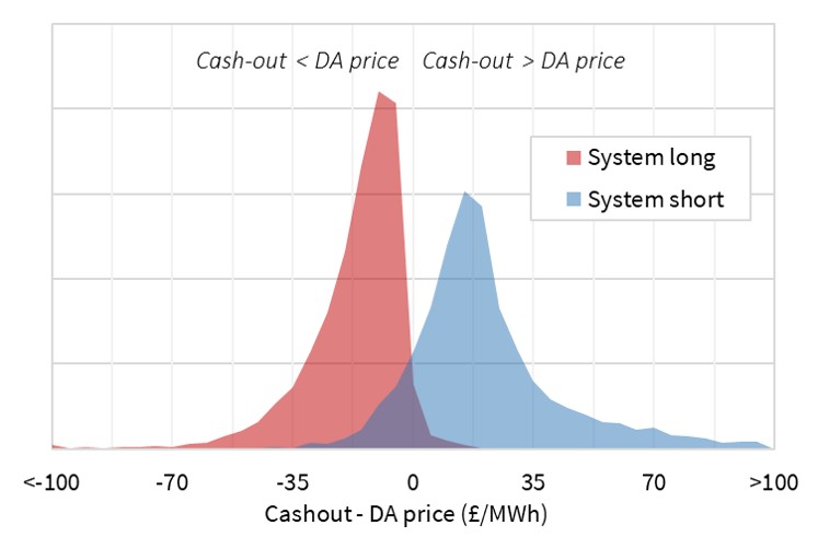
Source: Timera Energy
To develop the chart we have split price data into two buckets based on whether the system was long (red) or short (blue). This is easier to view than a combined distribution.
Take the blue distribution as an example. The expected differential between Day-Ahead and cashout prices was ~15 £/MWh (across periods when the system was long). But individual observed differentials fluctuated from -35 to +100 £/MWh. No matter how good your forecasting is, price swings that large cause forecasting errors that results in losses.
The sophistication of short term price forecasting techniques is improving rapidly (e.g. via applying machine learning). But as increasing volumes of battery (& engine) capacity are rolled out there are two factors making value capture more challenging:
- Value erosion: large volumes of flexible capacity responding to price signals in parallel may ‘cannibalise’ each other’s returns (a similar issue to that facing merchant wind & solar).
- Forecast error: price forecasting (particularly for cashout prices) is likely to become more challenging as volume swings from flexible capacity trying to capture prompt price moves increases.
These value capture challenges are not always robustly reflected in the quantification of battery economics. We return in our next article to look at the challenges investors face in quantifying battery value and building a robust investment case for merchant batteries.