LNG market evolution in 5 charts

Several key structural market trends are reshaping the way that LNG is transacted.

The US has emerged as a key provider of destination flexible supply, with almost 100 mtpa of committed export capacity.  Destination clause restrictions in existing supply contracts are also being relaxed or removed, helped by the negotiating balance swinging in favour of buyers in a well supplied market and competition authorities declaring these clauses anti-competitive.

Increasing demand uncertainty in traditional LNG markets is eroding appetite for long term and inflexible contracts. This uncertainty is being caused by evolving policy initiatives (e.g. the phasing out of coal & nuclear in Sth Korea), growth of renewable generation, ongoing market liberalisation and volume risk around Japanese nuclear restarts.

The rise of LNG portfolio players is rapidly eroding the traditional producer to supplier contracting model. This trend is being reinforced by the aggressive growth of commodity traders (e.g. Vitol, Trafigura & Gunvor) who are boosting market liquidity and shorter term contracting.

Reinforcing the trend to shorter contract durations, the next wave of LNG supply that is now taking shape is featuring the rise of equity offtake models (as opposed to long term contracts).  The recently FID’d LNG Canada project is a good example, where project developers will market their own equity share.

In today’s article we look at 5 charts that summarise the ongoing impact of these trends. The charts draw on data from the IEA’s recently published ‘Global Gas Security Review’.

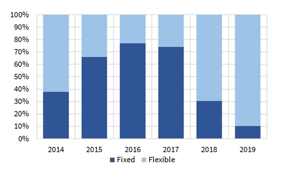
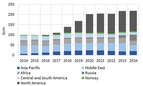
Chart 1: Growth of flexible destination clause contracts


Source: IEA

Chart 1 shows the level of destination flexibility in supply contracts concluded over each of the last 6 years. It includes contracts linked to FID’ed projects as well as portfolio sourced contracts.

The higher levels of flexibility in 2014-15 reflect the first wave of US export project FIDs. From 2017-19 a clear trend can be seen away from traditional fixed delivery point DES contracts towards greater diversion flexibility.

Contract duration has been falling in parallel, also reflecting the need for greater flexibility (although the 2018 FID of LNG Canada on an equity offtake basis somewhat skews recent stats). As long term DES contracts roll off, they are being replaced by destination free, shorter duration contracts. For example JERA sourced a 3 year, 2.5mt/year contract when its 15 year, 4.8 mt/y contract with Petronas ended in 2018.

Chart 2: Growth of gas – to – gas indexation


Source: IEA

Chart 2 shows the volume of gas indexed LNG supply volumes across the 2014-24 horizon (again including new projects and portfolio deals). A clear increase in gas indexation can be seen, with contract prices linked to traded hubs (e.g. Henry Hub, TTF, JKM) as opposed to traditional oil-indexation.

The rise of gas indexation reflects an increasing trust in gas price benchmarks as liquidity grows. It also reflects increasing mismatches between oil-indexed and end-user prices. There have been reports of coal indexed Asian LNG contracts, which is more logical than oil.

Chart 3: Growth of the portfolio player
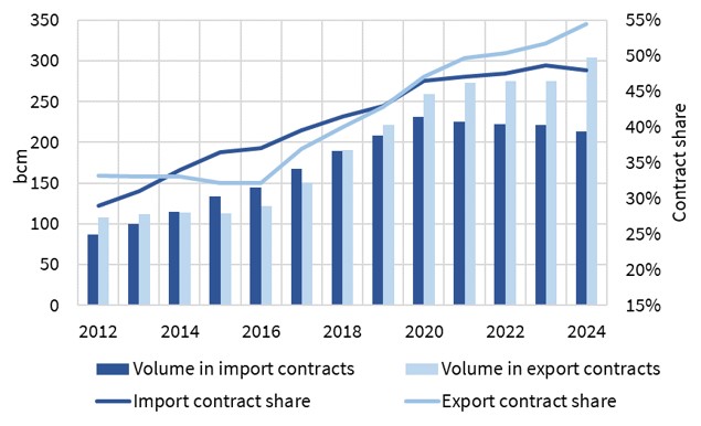

Source: IEA

The chart shows LNG contracts without a specific source (export contracts) or destination (import contracts). This provides a clear illustration of the rapid growth in the role of LNG portfolio players and the resulting breakdown in traditional producer source to supplier destination contracting.

Chart 4: Spot & short term share of total LNG trade


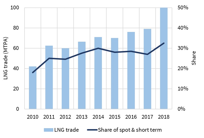
Source: GIIGNL, Kpler

As portfolio players disaggregate ‘bought’ from ‘sold volumes it creates a more complex portfolio optimisation & value management challenge. This is also creating a growing requirement for hedging, balancing & adjustment actions in the traded market, which is supporting liquidity growth.

This can be see in the rise in spot & short term LNG trade in Chart 4.  The rapid increase in flexible US export volumes coming online across 2018-20 should support this trend.

Chart 5: JKM swaps cleared through CME & ICE


Source: CME, ICE

LNG portfolio management is not just a spot problem. It is increasingly involving the forward hedging of portfolio exposures with financial products e.g. the hedging of gas indexed & diversion flexible US LNG contracts against TTF and JKM forward prices.

Chart 5 shows the rapid growth in volumes of JKM swaps across the last two years. Portfolio players are using swaps and futures to lock in prices on forward delivery volumes. These hedge positions can then be adjusted and optimised as market prices move, to manage risk and create value.

Five takeaways

In summary, the charts show 5 trends that are set to continue to shape the LNG market.

  1. Contracts are becoming more flexible & shorter duration
  2. Gas indexation is rising and replacing oil
  3. The role of portfolio players is growing, disaggregating source from destination
  4. As a result, spot & short term trading of LNG is growing…
  5. … and portfolio exposure management is also driving an increase in forward liquidity

These trends increase the complexity of the LNG market. But they also increase the ability to create value and manage risk.

The decarbonisation tipping point?

‘tipping point’: the point at which a series of small changes or incidents becomes significant enough to cause a larger, more important change.

Carbon dioxide concentration in the earth’s atmosphere has risen 40% since the industrial revolution. Half of that increase has occurred since 1980. And global carbon emissions continue to steadily rise.

There is clear scientific evidence of the link between rising carbon dioxide levels in the atmosphere and increasing average air & sea temperatures (see Chart 1). There is also growing evidence of feedback loops (e.g. melting sea ice) and accelerating changes in climate patterns, although these are more difficult to measure.

Scientific evidence is increasingly pointing to the fact that we are past the tipping point with respect to climate change.

The geopolitical implications of climate change are also coming into sharper focus. For example, the risks of large scale population displacement, decreasing availability of water & arable land and growing conflict for resources.  This increases the incentives for action.

So are we also reaching a tipping point in terms of a decarbonisation response?

This is the first in a series of two articles on a decarbonisation tipping point. Today we set out 5 drivers that suggest a tipping point could be upon us. Then in a second article we will look at the impact of more rapid decarbonisation on energy companies & portfolios.

Chart 1: Carbon emissions vs global average temperatures


Source: Global Carbon Project, NASA

5 drivers that suggest a decarbonisation tipping point is near

1.Lack of progress

Global carbon emissions rose 2% in 2018, the fastest pace for 7 years. This is despite plunging costs & rising volumes of renewable energy. The simple reason is that action on decarbonisation is being outpaced by emissions growth from rising energy consumption caused by population & economic growth.

The global population is increasing by about 1 million people every 4 days. Think of a mid-sized new city of energy demand created each week (as well as the other resources required to develop & support it).

In addition to population growth, economic growth in developing nations is increasing energy consumption of the existing population.  For example, 88% of the Chinese population lived below the poverty line in 1980 compared to less than 1% in today’s urbanised China. Energy consumption at the margin is still predominantly supported by fossil fuels.

The challenges of emissions reduction have seen the problem largely kicked down the road over the last 20 years. But scientific evidence is increasingly pointing to a window for action over the next 10 years in order to avoid more severe climate disruption. Discount factors are no longer enough to shrink the problem into the future.

2.Fiscal tailwinds

Austerity is dead. Long live Modern Monetary Theory (MMT).  There is growing momentum on both sides of politics to abandon austerity for fiscal expansion. Economists as well as politicians are swinging behind fiscal spending, led by central bankers who are confronted by the limits of monetary policy in propping up economic growth.

The basic premise of MMT is that in a low inflation environment, deficits don’t matter so long as a country can print money in its own currency. Modern Monetary Madness? Maybe… but in a world struggling against powerful demographic & technology driven disinflationary forces, MMT is a seductive economic narrative to justify political spending.

Countries with this ability to monetise their own debt (e.g. US, Europe, Japan, China) look increasingly likely to embark on large fiscal spending programs. Decarbonisation is an obvious spending target, as evidenced by the rise of the ‘Green New Deal’ in the US.

The costs of large scale decarbonisation are also falling with rapidly declining borrowing costs. Interest rates on government & corporate debt have plunged in 2019, continuing a 40 year downtrend. There is now more than $15 trillion of negatively yielding debt worldwide (i.e. lenders paying borrowers to take their money away). The combination of targeted fiscal spending & low rates may create powerful tailwinds for decarbonisation.

3.Business is engaging

There has been a subtle but important shift of big companies behind decarbonisation over the last 2-3 years. This is in part in response to the rising importance of climate change to customers.  Global giants such as Google, Microsoft and Unilever are decarbonising their business models at a much faster pace than policy requires. Many large companies have now set (or already achieved) 100% electricity decarbonisation targets and are looking to expand on these.

But there are much larger economic incentives in play. Large tech & consumer companies see growing fiscal, technology & decarbonisation tailwinds as an opportunity to disrupt traditional energy companies (e.g. utilities & oil majors) & supply chains. Energy companies are also actively repositioning for growth from decarbonisation, as are engineering firms tackling resilience projects (e.g. sea walls).

This trend of business support for decarbonisation helps smooth the way for more aggressive policy action.

4.Generational mobilisation

Greta Thunberg, a 15 year old Swedish girl, started a one person ‘climate strike’ in August 2018. A little over a year later she was favourite to win the Nobel Peace Prize going into the ceremony last week (although it went to the Ethiopian PM) . What makes her impact larger than the many other people who have tried similar protests over the last 20 years? Timing would appear to be an important factor.

Whatever you think of Greta’s political influences, she symbolises the rapid mobilisation of a generation in a way not seen since at least the 1960s. 2019 has seen large youth climate protests on an almost daily basis, involving millions of people from a broad range of countries, wealth levels and political backgrounds.

This organic climate movement is hard to pin down. It seems to capture a complex (and sometimes inconsistent) mix of issues, politics & proposed solutions.  But there is one common theme that binds the movement together: a demand for climate action now.

5.US leadership?

The Democrats are now odds on favourites to win the White House in 2020. Trump’s odds of winning are slipping with the fortunes of his ‘greatest economy in history’ (he is now 11/8 to win a second term).

It is unclear which of the Democrat candidates will take on Trump. But fiscal expansion to support the Green New Deal is a prominent policy goal for all of the leading Democrats. A Democrat in the White House could see the full force of US innovation thrown behind decarbonisation.

Even in the absence of a Democrat President, there has been growing decarbonisation momentum at a state level. 16 states have now committed to 100% renewable or 100% carbon free targets by 2050.  California (the 6th largest economy in the world) is playing a particularly important role in implementing policy change.

Clear US leadership on decarbonisation over the next five years would likely precipitate a rapid acceleration of the global response.

What does this mean for European energy?

We have become used to a relatively slow rate of progress on decarbonisation over the last 20 years. That could of course continue. There is still considerable inertia acting against rapid change.

But the five factors above are increasing the probability of a step change in decarbonisation response across the next 5-10 years.

Current trends point to this response being led by:

  1. Developed countries
  2. Europe (as a subset of developed countries)
  3. The power & gas sectors.

That means European power & gas markets are likely to be at the epicentre of global change. They are the low hanging fruit.

We consider the implications of accelerated decarbonisation on energy companies & portfolios in the next article.

Gaining an edge: LNG portfolio analysis

Commercial evolution of the LNG market has accelerated over the last three years. This is the result of new and more flexible sources of supply.  But it also reflects new market players, rising liquidity and a transition to shorter & more flexible contracting. As the LNG market grows and matures, substantial value creation opportunities are emerging.

These opportunities are reflected in the evolution of LNG market players. Big producers (e.g. Shell, BP, Total) are expanding their value chain presence. Trading focused intermediaries (e.g. Vitol, Gunvor, Trafigura) are driving liquidity growth and evolution of the traded market. Large buyers (e.g. JERA, Kogas, Pavilion) are expanding their portfolio footprints and developing commercial capabilities or JVs to support this growth.

One of the foundations of successful value creation is a robust commercial analysis framework, to tackle:

  1. Shorter term optimisation of portfolio flexibility, constraints & logistics
  2. Management of portfolio value via hedging & structured deals
  3. Creation of incremental portfolio value via new assets/LTCs or M&A
  4. Risk management of portfolio exposures

A successful analytical framework plays a key role in gaining a competitive edge when building and optimising an LNG portfolio. In today’s article we set key challenges and success factors in developing a solution. This draws on our first hand practical experience working with some of the largest players in the market to develop their in-house solutions.

5 key challenges of LNG portfolio analysis

Building an effective LNG portfolio analysis framework means confronting several key challenges.

1.Value chain interdependence

In many markets, liquid prices mean that portfolios can be valued and managed at an individual asset level. This is not the case with LNG portfolios. The value of LNG assets within a portfolio is interdependent, given the physical & contractual complexity of the LNG supply chain. As a result, valuation & optimisation needs to be tackled on a portfolio basis, recognising asset interactions & constraints.

2.Bespoke business models

Each LNG business model & portfolio has bespoke analytical requirements.  These relate to the specific exposures, constraints & logistics of portfolio components. Requirements are also driven by the business model of the portfolio owner e.g. ‘trader’ focus on building portfolio optionality, ‘buyer’ focus on managing physical supply. The bespoke nature of the problem undermines the effectiveness of ‘off the shelf’ analytical solutions.

3.Illiquid markets

Despite rapid growth, the LNG market remains relatively illiquid & has complex physical & contractual logistical constraints (e.g. shipping, ports, canals, pricing & volume flex).  This creates challenges in valuing & hedging complex (e.g. non linear) exposures. But these liquidity constraints also lie at the core of value creation opportunities. A transparent but robust deconstruction, optimisation & valuation of complex exposures underpins an effective analytical solution.

4.LNG price behaviour

LNG prices are not normally distributed!  Standard pricing models do not capture complex relationships across LNG price markers. For example, the levels of price spreads, volatility & correlation depend on the prevailing ‘regime’ of the market.  Pricing dynamics in a well supplied market tend to reflect convergence, high correlations and low volatility.  In a tight market, prices temporarily diverge with correlations falling and volatility rising. Getting price analysis right can generate big competitive advantage.

5.Lack of standardised methodologies

Because of the 4 issues we set out above, there is a lack of standardised methodology for LNG portfolio analysis.  As a result, companies are developing bespoke solutions. But a consistent approach is evolving across a number of the key analytical building blocks required (e.g. formulation of constraint problems, valuation approach for specific types of optionality). This is breaking down the barriers to developing an effective solution.

If those are the 5 key challenges, what are the success factors underpin a solution?

Creating & analysing LNG portfolio value

How is value created?

The most accurate answer is probably… in a pub over a ‘five o’clock’ beer.

But behind the deals that underpin a portfolio, value is created via the interaction between:

  1. Constraints & stress points in the LNG supply chain
  2. Changes in market dynamics.

Value is captured via constructing & optimising an appropriate combination of portfolio components & optionality. Understanding the way that portfolio value is practically created and monetised is the most important success factor in building an effective analytical solution.  There is some important theory behind this, but theory on its own is useless.

How is this represented analytically?

LNG portfolios can be simplified using market price ‘nodes’ and asset ‘exposures’.  Market prices act on exposures to drive portfolio value. Diagram 1 shows a simple illustration of key LNG market price nodes. Diagram 2 summarises some key LNG portfolio exposures.

Diagram 1: An illustrative representation of key LNG price nodes


Table 1: Breakdown of some key LNG portfolio exposures


Source: Timera Energy

An effective analytical representation of an LNG portfolio is built on the definition of:

  • Nodal price dynamics (price level, spreads, correlations, volatility), ref Diagram 1
  • Portfolio exposures (e.g. commodity positions, asset flex & constraints), ref Table 1.

If you can define a realistic but transparent representation of the way price dynamics act on exposures, you are more than half way to cracking the problem.

Choosing the right weapon for the hunt

An effective analytical capability to support an LNG portfolio usually covers four distinct areas. These are summarised in Diagram 2.


Source: Timera Energy

There is a natural temptation to acquire an ‘elephant gun’ to tackle all four areas at once.  This is a big mistake in our view.  There can be common building blocks and a consistent approach, but a ‘one size fits all’ solution ignores the different nature of these four problems.

For example, an analytical tool to support prompt optimisation of portfolio cargo routing & logistics over a 6 month horizon, requires portfolio components & constraints to be represented in very granular detail.

It is ineffective and restrictive retaining that level of detail when analysing value management or portfolio construction over a 2-10 year horizon. Over this horizon, focusing on the impact of commodity price uncertainty is much more important than capturing detailed logistics.

The value of prototyping

Most players in the LNG market are developing their own in-house solutions. This reflects the pitfalls in trying to buy & configure an ‘off the shelf’ solution (as described in the 5 key challenges section above).  A well constructed analytical solution can be a unique source of competitive advantage. It can literally pay for itself in a day, via increased value capture.

A key challenge in developing such a solution is effectively defining requirements and approach. It is very hard to do this in a ‘one shot’ upfront design phase. This is where we have found a simplified ‘proof of concept’ can substantially improve results and reduce costs.

The objective of this proof of concept approach is to build a functionally rich and commercially robust working prototype of the enduring analytical solution. This allows:

  1. Practical engagement with business users (e.g. originators, traders)
  2. More effective iterative definition of requirements & methodology
  3. Flagging of any major issues and the flexibility to address these
  4. Early & valuable insight into how analytical results can practically be applied in supporting commercial decision making.

Many elements of the proof of concept can often be efficiently adapted into part of the enduring solution.

For more details on how to tackle the development of an LNG portfolio analysis capability, we have included a link to a briefing pack below.

Briefing pack: LNG portfolio value
Sep 2019 Timera briefing pack with approaches and case studies on identifying & capturing LNG value: Gaining an edge


European gas storage value is recovering

Three structural drivers are tightening the gas flexibility balance across Europe:

  1. Rising import dependency: resulting in a reliance on longer & less flexible supply chains (e.g. LNG, Russian pipeline gas)
  2. Power sector transition: with rising renewable intermittency and the closure of nuclear & coal plants increasing the role of gas-fired power plants in providing flexible generation
  3. Ageing infrastructure: investment in new flexible midstream gas assets has ground to a halt over the last 5 years, with owners ‘sweating’ existing assets.

In today’s article we set out clear evidence of a recovery in gas flexibility price signals across 2018-19. We also show ‘backtesting’ analysis that illustrates how price signal recovery is translating into higher value capture from storage capacity.

Price signals recover… at last

The value of gas flexibility (e.g. from storage, production & pipeline flex & regas) is driven by two key market price signals:

  1. Spot price volatility drives the value of deliverability (i.e. flexibility response near to delivery)
  2. Seasonal price spreads drive the value of seasonal flexibility.

Chart 1 shows the evolution of these two price signals since 2016 at Europe’s core TTF hub.

Chart 1: Evolution of day-ahead TTF volatility (left) & front year seasonal spreads (2016-19)


Source: Timera Energy, ICE data

The left panel of the chart shows a clear recovery trend in TTF spot volatility since 2017. Volatility has averaged above 70% so far in 2019 (& is currently above 100% on a 30 day rolling basis). It is interesting to note that this rise in volatility is happening against the backdrop of a well supplied gas market and lower prices.  A key driver of higher volatility over the last 12 months has been the role Europe has been playing in absorbing surplus LNG cargoes to balance the global market.

The right panel of Chart 1 shows the forward TTF summer/winter spread as it evolves in the lead up to each storage year (Apr to Mar). A rise in seasonal spreads can arise from three situations: (i) an increase in winter prices, (ii) a fall in summer prices and (iii) both of these factors combined.

Fears around winter tightness are the most common cause of rising spreads. But in 2019 the focus has been on summer price weakness, given a requirement to clear high volumes of LNG imports. This caused the Sum-19 / Win-19 spread to surge across Q1 2019.  And the recovery in spreads has also fed through into Sum-20 / Win-20 price spreads, which are around 2.3 €/MWh, almost double the levels of last year.

It is worth noting that price signal recovery at the UK NBP has been sharper given the impact of the retirement of Rough storage in 2016.

Storage margins follow suit

It is no surprise that price signal recovery has translated into higher potential returns for storage capacity holders. Although the level of storage margin capture for any given capacity owner depends factors such as inventory levels and forward hedge positions.

In order to provide a simple benchmark on value recovery we have ‘backtested’ margin capture for a generic fast cycle (60 day cycle) and seasonal (180 day cycle) storage asset. The results across each of the last 4 storage years are shown in Chart 2.

Chart 2: Backtest of margin capture for fast cycle (left) and seasonal (right) storage assets


Source: Timera Energy

We use our in-house storage modelling framework to do this, applying a commonly used rolling intrinsic trading strategy.  This involves analysis of margin capture from actual (or ‘outturn’) market price movements where hedges are adjusted against available forward contract prices as these evolve.

Fast cycle margins have recovered by a proportionally higher amount than seasonal asset margins. This reflects the leveraged exposure of fast cycle assets to the recovery in volatility.  But there has also been a significant increase in seasonal asset value capture across the last two years, as both volatility and spread recovery lifts returns

Who will benefit from value recovery?

In the short term, the benefits of rising storage margins have been skewed towards capacity buyers e.g. trading desks.  This is because buyers have bought storage capacity from asset owners at price levels that reflect the weaker market conditions that preceded the recent price signal recovery.

A continuation in storage value recovery should increasingly flow through to asset owners (vs buyers).  This is because increasing volumes of storage capacity are being sold on an annual (or shorter term) basis, as long term contracts roll off and are not renewed.

However the ability of storage owners to maximise value capture depends strongly on capacity sales strategy, contract structures and business model.  We explore these factors alongside drivers of continuing storage value recovery in a recent briefing pack (link below).

Briefing pack: European Gas Storage Value
Sep 2019 Timera briefing pack on gas storage margin recovery, market drivers & commercial implications.: Gas storage value recovery


German & Dutch CCGT value case

Between 2005-10 there was a mini boom in CCGT investment in Germany and the Netherlands. These projects reached FID against a backdrop of relatively healthy gas-fired generation margins (spark spreads). But by the time CCGTs were commissioned, owners were confronted by a relentless decline in margins.

Renewable penetration gathered pace eroding CCGT load factors.  Large new & efficient coal plants also came online, with falling coal and carbon prices increasing the competitive advantage of coal vs gas plants.

But the most pronounced value hit for CCGTs came from the erosion of electricity demand as a result of the global financial crisis.  With CCGTs on the margin in most markets, falling demand translated directly into falling load factors & margins.

CCGT values & spark spreads plumetted across 2010-15.  But margins started to stabilise in 2016 as gas for coal plant switching gathered momentum. The last 12 months have seen further CCGT margin improvement as European hub prices plummeted. And capacity mix changes over the next 3 years point to a more structural margin recovery.

Today we summarise what we think is an interesting contrarian investment case in existing German & Dutch CCGTs, targeting a 10 year horizon.

Gas for coal switching has driven margin recovery

Between 2010 -2015, relatively low coal & carbon prices underpinned a structural variable cost advantage of coal plants over CCGTs. Clean spark spreads were negative, even on a peak basis, as shown in Chart 1.

Chart 1: Peak German Clean Spark Spreads & current forward curves


Source: Timera Energy, ICE

As a result CCGTs, many of which were newly commissioned, were effectively demoted to a peaking backup role.

The 2016 slump in gas prices started a recovery in sparkspreads and CCGT margins. This margin recovery reversed to some extent across the first three quarters of 2018 as gas prices rose again.  But since Q4 2018 there has been a further sharp increase in CCGT generation margins, with plants running predominantly baseload across Summer 2019.

The volatile nature of spark spreads illustrates why it is tough to build an asset investment case on market price views alone.  So are there other structural drivers supporting CCGT margin recovery?

Sweeping NW European capacity closures

The German power market is facing almost 25GW of regulatory driven plant closures over the next 3 years. This is a combination of closure of the nuclear fleet and closure of hard coal & lignite to meet Coal Commission targets.

But Germany is not unique. Coal & nuclear closures are a theme across NW Europe. Chart 2 provides a summary of of cumulative regulatory driven closures across NW Europe.  These numbers are large: 30GW by 2022, more than 60GW by 2030 (and this does not include ‘end of life’ closures of ageing CCGT plants).

Chart 2 Cumulative regulatory driven closures of NWE coal & nuclear plants


Source: Timera Energy

The scale of closures over the next 3 years will significantly tighten the German and NW European power market balance.  Gas-fired plants are set to take up the slack, transitioning to dominate the setting of marginal power prices. In other words, capacity closures will structurally increase gas-plant load factors.

Building a CCGT investment case

There is a well-worn narrative as to why investment in NW European CCGTs is a bad idea: ‘Renewables deployment erodes margin… Decarbonisation risk is growing… Margins are volatile & commodity price dependent…  And look at the writedowns owners have suffered over the last 5 years!’.

All of the elements of this narrative are undeniably true. But an asset investment case depends on the relationship between risk adjusted returns and asset acquisition cost.  A strong consensus narrative is typically reflected in asset prices.

So let’s turn the problem on its head and approach it by defining a set of 5 drivers that could underpin an investment case:

  1. Motivated sellers: Utilities have taken CCGT writedowns. They are also strategically shifting business models away from owning thermal power assets. Relatively new assets have transacted for cents in the dollar (vs build cost).
  2. Buying optionality: CCGT acquisition can be thought of as buying spark spread optionality. After a tough decade, this optionality is now back ‘in the money’, reducing the risks & costs of value capture. This optionality means asset owners are long volatility… in an environment of rising renewables & structurally tightening energy & capacity balances.
  3. Barriers to entry: Retaining existing CCGTs is the cheapest form of incremental system flexibility (outside specific applications for short duration batteries). The biggest margin threat for existing CCGTs is new CCGT build… but the investment case for new CCGTs just gets tougher as decarbonisation risks grow.
  4. Defined timeline: Plant closures over the next 3 years are not a hypothesis – they will almost certainly be implemented (with German efficiency). That underpins a clear 5 year margin recovery case & target payback window.  It is easy to under-estimate further optionality & upside value beyond this (e.g. via introduction of explicit or implicit capacity payments).
  5. Decarbonisation: It is brave to bet against decarbonisation given the current policy momentum in Europe. Yet the more action accelerates, the faster the closure of coal and the bigger the hurdles to new CCGT build. Over a 5-10 year horizon, CCGT owners are long decarbonisation.

Now to dampen all the enthusiasm with a very practical caveat. Not all CCGTs are created equal – the right flexibility, location & plant cost structure are key to making the numbers work.

Inter-market shock roils power, TTF & JKM

In our snapshot column last week we flagged a huge rally in power & gas forward curves. The move was driven by three announcements that surprised bearishly positioned markets last Tuesday.

The most important of these was EDF flagging potential new safety issues with its French nuclear fleet. Markets may have short memories, but not short enough to have forgotten the nuclear fuelled fireworks of Winter 2016-17.

Reinforcing the gas market impact of the EDF announcement, the Dutch government further tightened the production cap on the giant Groningen field and announced the end of production by mid 2022.

The third surprise came from the ECJ, which ruled that Gazprom access to the key OPAL pipeline into Germany will need to fall back to 50% of capacity.

Price rises and volatility are likely to continue into this week. The US has blamed Iran for a weekend drone attack that has temporarily crippled more than half of Saudi Arabia’s oil production (~5% of global supply). A very volatile front month Brent contract has been trading 10-20% higher than Friday since the market opened today.

3 factors behind last week’s market moves

French nuke risk

EDF has flagged ‘a deviation from technical standards’ relating to welds on the steam generators of some of their nuclear reactor fleet. The initial EDF statement provided little clarity on how many reactors may be impacted and what the timing of any outages could be.

The French nuclear authority (ASN) subsequently announced that at least 5 reactors had been impacted, with a more detailed statement expected from EDF in the coming week. The resulting uncertainty has seen a significant risk premium driven into French winter power prices, although the impact of outages this winter is unlikely to be as dramatic as in Win 16-17.

Groningen cuts

5 years ago the giant Groningen field in the Netherlands was producing more than 40 bcma of gas. Since then the Dutch government has consistently reduced the production cap on the field given increasing concerns over ongoing earthquakes. The cut announced last week caps gas production at less than 12 bcm for the coming gas year. By mid-2022 output will now fall to zero.

Production cuts had already been flagged earlier this year. But last week’s announcement was at the higher end of market expectations.  This helped support a rally across the TTF gas curve, although the big surge in gas prices was more focused in Win-19 given the French nuclear issues.

Gazprom OPAL access  

The ECJ ruling last week overturns a 2016 decision to allow Gazprom access to up to 80% of the OPAL pipeline that links Nord Stream to Germany. This effectively returns the 50% cap on Gazprom’s use of OPAL, reducing its ability to flow gas via the Nord Stream/OPAL route by 12.5 bcma.

This volume can flow via the Ukraine/Slovakia route instead. So it is unlikely to result in any immediate supply cuts to Europe. But it shifts the balance of negotiating power towards Ukraine for the very important transit agreement talks that are underway.  The transit agreement that allows Gazprom to flow gas via Ukraine (one of its 3 key access routes into Europe) is due to expire at the end of this year.

How has this impacted market prices… so far?

The triple shock that hit markets last week is a great case study in the increasing importance of inter-market linkages. In an energy market version of the butterfly effect, the risk of nuclear outages in France immediately flowed through to higher JKM LNG prices in Asia.

The logic? Nuclear outages in France are ‘backfilled’ primarily by incremental CCGT output (both within France and from neighbouring countries). The implied increase in gas demand dragged up TTF prices, with a knock-on impact across other European hubs. This in turn was transmitted to Asian LNG prices which are underpinned by TTF as European hubs support a well supplied global LNG market.

French power prices for the coming winter rose 12% last Tuesday as the risk of rolling nuclear outages lifted the curve. Power market curves across NW Europe were pulled higher in sympathy (e.g. in UK, Belgium, Netherlands & Germany).

The move in gas prices was almost as pronounced, with Win-19 TTF prices rising around 10%. While the price surge at European hubs was focused on the current winter, the whole gas curve moved higher as shown in Chart 1. This was in part due to bearish positioning after relentless price declines across 2019, but was also helped by the Groningen & OPAL announcements which may have more enduring implications for European gas supply.

Chart 1: One day TTF gas curve move (Tue 10th Sep)


Source: Timera Energy

The events of last week were also supportive of the ongoing rally in NW European CCGT margins. French spark spreads showed particular strength, consistent with a rising forward price signal for CCGTs across the coming winter.

5 things to watch going forward

We finish by flagging 5 factors to watch as a result of the 3 announcements last week:

  1. Win 16-17 revisited: Risks for this winter look less extreme than the shocks of 3 years ago, but recent history shows that it pays to be adequately insured i.e. don’t be caught short flex.
  2. CCGT margins: Price moves last week reinforce the recovery in European gas-fired generation margins we wrote about last week. Nuclear outages are bullish for gas asset margins.
  3. Low Cal constraints: The rapid pace of decline in Groningen’s Low Cal gas production is resulting in a rapidly growing requirement for Hi to Low Cal conversion capacity. Any constraints over the next 3 years may cause price divergence.
  4. Ukraine flows: The OPAL decision will cause flow rerouting & may see Ukraine push Gazprom harder in transit talks into year end. Any disruption of flows via Ukraine this winter will now have a bigger impact.
  5. Gas market balance: Higher CCGT burn & Groningen cuts support Europe’s ability to absorb surplus LNG across next 1-2 years. This may help with the rebalancing of the global LNG market from its current state of oversupply.

In addition there is the wildcard impact of the Saudi attacks on the oil market.  Oil is not as direct a driver of European gas & power markets as it used to be given the rapid reduction of oil-indexation in gas contracts.  But a disruption of this scale in the oil market will introduce both upward price pressure and volatility to the gas market.  Winter 19-20 is shaping up to be anything but boring.


Major shifts in German power pricing dynamics

Renewable output is growing fast across North West European power markets. Wind & solar output in Germany accounts for more than 30% of demand. Include other renewables (e.g. hydro & biomass) and this share rises to more than 40%.

Rising renewables penetration is resulting in an increasing number of periods where thermal plants are completely displaced in the merit order. During these periods, power prices can temporarily plunge to low or even negative levels as other forms of lower variable cost capacity set prices (e.g. nuclear, biomass or wind).

Despite rising price volatility associated with intermittency, CCGT and coal plants remain the dominant driver of power prices across NW Europe. Even with a 40% renewable market share in Germany, thermal plants are setting the power price most of the time (sitting on the margin above wind & solar output in the stack). This is particularly evident in the very strong forward curve relationship of power prices versus gas, coal & carbon prices.

It is this forward curve relationship that we look at today.  Some major shifts in the relative costs of gas & coal plants in 2019 are having an important impact on the evolution of power prices and generation margins. These are in turn causing a shift in competitive balance and generation asset returns.

4 charts tell the story

Spark and dark spreads are a benchmark for the generation margins for CCGTs and coal plants respectively (power price minus variable cost).  These spreads provide an important insight into power market pricing dynamics.

The top two panels in Chart 1 show Baseload & Peak German forward Clean Spark Spreads (CCGT margins) in Germany across the last 18 months. The bottom two panels show Base & Peak Clean Dark Spreads (coal plant generation margins).  The 3 lines on each chart show:

  1. Light blue = Summer 2019
  2. Grey = Winter 2019/20
  3. Darker blue = Summer 2020

Chart 1: Base & Peak German CSS (top 2 charts) & CDS (bottom charts)

Source: Timera Energy

Winter

CCGTs are the dominant setter of marginal power prices across the winter.  This is reflected in a relatively stable CSS level (grey line in the top panel). As gas prices have declined over the last 12 months, CCGT variable costs have fallen and this has fed through into lower power prices. In other words, falling gas prices have been dragging power prices lower.

The bottom panel show how falling gas prices have also been hurting coal plants. Lower power prices are feeding through into lower CDS, with Baseload Win 19-20 CDS falling by 50% since Q4 -18 (from 8 €/MWh to just above 5 €/MWh).  Coal plant load factors and margins are following suit.

The ‘market’ CDS shown in Chart 1 do not include coal transport costs, which further reduce achieved dark spreads. These vary by asset, but range from 2 to 8€/MWh.

Summer

Lower gas prices across summer periods have seen coal plants relegated to a peaking role. This is reflected by a relatively stable Peak CDS across Sum-19 and Sum-20.

The influence of higher variable cost coal plants supporting summer prices has been good news for CCGTs. The top two panels show a big recovery in CCGT generation margins across summer periods as gas prices have fallen across the last 12 months. Lower gas prices are translating into higher CCGT load factors and higher margins.

At the start of Q4-18, Baseload CSS was deeply negative (- 7 €/MWh for Sum-19, – 12€/MWh for Sum-20). Even Peak CSS was hovering around zero. In other words CCGTs were structurally ‘out of the money’ on a forward price basis.

Since then Baseload CSS has surged into positive territory, with Peak CSS rising to around 8 €/MWh for Sum-20 (yes that’s with a positive sign in front of it!). In other words CCGTs are structurally back ‘in the money’ across both next winter and summer.

What does this mean going forward?

We use Germany to illustrate spread and price formation dynamics as it sits at the core of the interconnected network of North West European power markets. But the same dynamics are impacting neighbouring market (e.g. France, Netherlands & Belgium).

The shift that has taken place in relative fuel prices means that power prices across NW Europe have become more strongly linked to gas prices, and less influenced by coal. This reinforces the importance of the gas market in understanding power price dynamics.

The other dynamic that is occurring, almost under the radar, is a significant recovery in CCGT margins in NW Europe. After almost a decade of margin erosion and asset writedowns, CCGTs are in the money again.

The CCGT value recovery story could have more to run. There are some important structural drivers that are set to support CCGT load factors and margins over the next 3-5 years. We will address the evolution of CCGT value soon in a follow up article.


Building a viable battery margin stack

We flagged a ‘take off’ in European merchant battery investment as one of our 5 surprises to watch out for in 2019. Investment momentum has been accelerating as the year progresses, and merchant business models have become the dominant focus.

Investment in Europe is being led by the UK and German power markets, with high renewables penetration and a more constructive policy environment supporting battery projects. Merchant investment is being fuelled by a combination of utilities (e.g. EDF, Uniper, Centrica), funds (e.g. Gresham House & Gore Street) and a range of renewables investors looking to pair batteries with solar, wind & other innovative strategies.

But battery investors all face a common challenge: building a viable margin stack that will underpin a return on capital. This is significantly more challenging for battery projects than for renewable or conventional thermal asset investments because of:

  1. Margin sensitivity to rapidly changing market & regulatory conditions (e.g. capacity mix changes & policy evolution)
  2. The complex nature of battery optimisation, across different markets and time horizons, to capture wholesale market margin
  3. A lack of historical data on achieved battery margin performance

One of Timera’s key focus areas this year has been working with battery investors on quantifying robust margin cases. In today’s article we outline our view on how to approach the analysis of a viable margin stack.

Breaking battery margin into buckets

The complexity of battery margin capture means it is imperative to develop a way for investors to understand margin build up, without requiring a double PhD in maths & physics. In our view, the best way to achieve this is to break margin down into buckets as shown in Chart 1.

Chart 1: Battery margin buckets & capability required to capture value


Source: Timera Energy

  1. Base margin: The merchant margin stack is underpinned by non-wholesale market margin streams. These include system services (e.g. frequency response, reactive power), capacity payments and project specific site/locational benefits. The advantage of these margin streams is that they are typically less risky than wholesale market margin and may even support some project debt.
  2. Structural price shape: Power markets have a structural intra-day price shape driven by the variable costs of different capacity types setting prices across the day. A lower bound for battery wholesale margin can be generated based on arbitrage of this structural intraday price shape e.g. via a simple rolling intrinsic strategy. Rising renewables penetration and retirements of coal / nuclear / CCGT plants is acting to increase price shape over time, supporting value in this bucket.
  3. Structural volatility: The very fast reaction speed of batteries in response to price volatility underpins battery wholesale margin capture. There is an inherent underlying level of prompt price volatility (or ‘price noise’) in power markets caused by fluctuations in load, wind and solar. This is increasing with renewables penetration. Value capture is riskier and more complex than for simple arbitrage strategies, but there are formulaic or algorithmic methods to ‘harvest’ value from this volatility without incurring high risk.
  4. Additional volatility: The final margin bucket is made up of riskier extrinsic value. This depends on how much additional price volatility occurs in the market above the inherent ‘price noise’ in bucket 3. Drivers include periods of market tightness and market events such as weather shocks & outages. The amount of value captured here has a stronger dependence on trading capability & commercial judgement.

Interpreting the margin buckets

The portion of value that sits in each of the four buckets varies significantly by commercial strategy, project configuration, location and market. The levels achievable in buckets 1 to 3, determine how much margin must be generated via the higher risk bucket 4, in order to meet required return on capital.

These buckets are very useful in building up a ‘digestible’ view of battery margin analysis. But they are not a way to side step what is a very complex analytical problem behind. The wholesale margin buckets 1 – 4 can be shown separately on a diagram, but are in practice co-dependent. Value is captured via an all-inclusive optimisation of battery flexibility across multiple time horizons. So what analytical tools are required to do this justice?

Quantifying margin bucket value

Firstly, it is important to specifically capture wind, solar & load uncertainty within the market modelling process. It is imperative that these factors are properly simulated (e.g. 500+ simulations) in order to understand their impact on market price volatility.

This means applying a stochastic power market modelling framework (follow the link for an explanation).  Traditional ‘Base / High / Low’ scenario analysis of power prices is not appropriate for quantifying battery margins.  This approach tends to underestimate both battery value capture and market risk.

Secondly, it is important to model battery margins using a robust stochastic battery optimisation model. This is a separate tool from the stochastic market model.  It captures optimisation of battery dispatch against wholesale market prices, including the variable cost impact of battery cycling degradation and bid/offer spreads.

A robust market & margin modelling framework underpins an understanding of how batteries can practically create margin. More importantly it helps quantify the risk dynamics around projected margins.

3 new members join our growing Timera team
Jon Brown joins us from EDF, Steven Coppack from Total & Tommy Rowland from Smartest Energy. As with all of our team members, they have a strong practical background in commercial analytics from their industry roles. More details on Steven, Jon & Tommy on Our Team page.Timera Energy also move into new offices this week: L12, 30 Crown Place, London EC2A 4ES – details here.